Properties of Laplace Transforms

PROPERTIES OF LAPLACE TRANSFORMS

The Following are the Properties of Laplace transform,

(i) Linearity

(ii) Shifting Theorem (or) Translation in Time Domain

(iii) Complex translation (or) Translation in Frequency domain

(iv) Differentiation theorem (or) Differentiation in time domain

(v) Integration Theorem

(vi) Initial Value Theorem

(vii) Final Value Theorem

(viii) Laplace Transform of a periodic Function.

(ix) Convolution Theorem

(x) Time Scaling

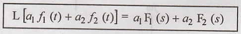
Linearity

Let f₁(t) ↔ F₁(s) and f₂(t) ↔ F₂(s) be the two Laplace Transform pairs.

Then linearity property states that,

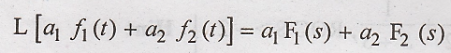
Here a₁ & a₂ are constants.

To Prove:

Proof :

Let us find the Laplace transform of a1 f₁(t) + a₂ f₂(t) by applying the definition, (ie)

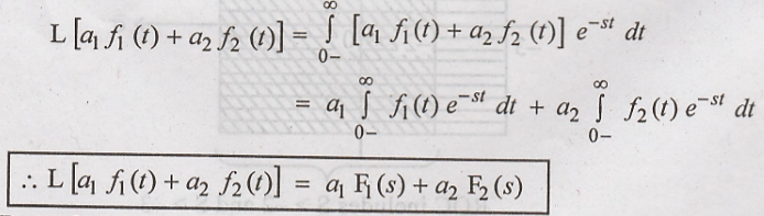
Hence Proved.

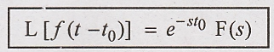
Shifting Theorem (or) Translation in Time Domain

Let f(t) ↔ F(s) be a laplace transform pair.

If f(t) is delayed by time (t₀), then its laplace transform is multiplied by e ^{– s t}₀

Proof :

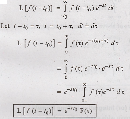
Hence Proved

Complex Translation (or) Translation in Frequency Domain

Let f(t) ↔ F(s) be a laplace Transform pair.

A shift in the frequency domain is equivalent to multiplying the time domain signal by complex exponential.

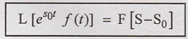
Proof:

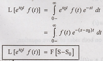
Hence proved.

Differentiation Theorem (or) Differentiation in Time Domain

Differentiation in time domain adds a zero to the system.

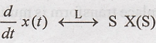
Proof:

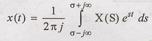
Differentiate both sides of above equation with respect to 't'.

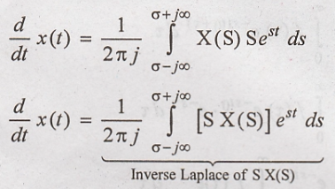
Hence Proved

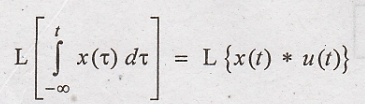
Integration Theorem (or) Integration in Time Domain

Integration in time domain adds a pole to the system.

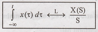
Proof :

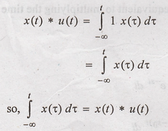
Taking Laplace transform on both sides of above equation,

Hence Proved

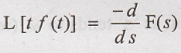
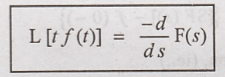
Differentiation By 'S'

L[f(t)] = F(s). Then differentiation in complex frequency domain corresponds to multiplication by 't' in the time domain. (i.e.,)

To Prove:

Proof:

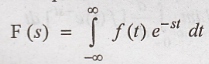
By definition of Laplace transform

Differentiate the above equation with respect to S, (ie.,)

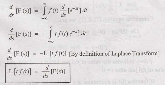
Hence Proved

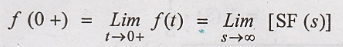
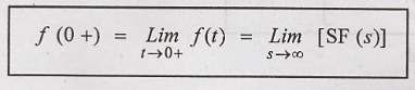
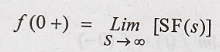
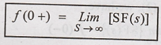
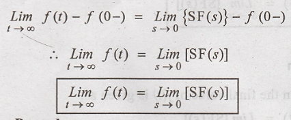
Initial Value Theorem

If L[f(t)] = F (s), then initial value of f(t) is given as,

Where the first derivative of f(t) should be Laplace transformable.

To Prove:

Proof :

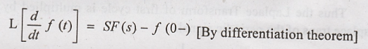
We know that,

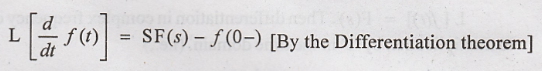
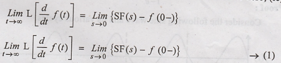
Let us take limit of the above equation as 's' tends to ∞ (ie.,)

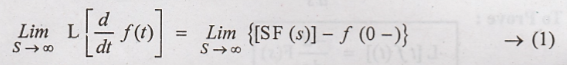
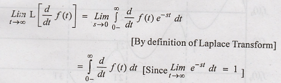
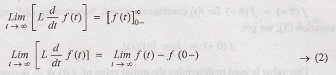
Consider LHS of the above equation, (ie.,)

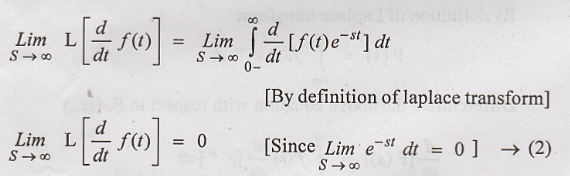
Comparing equation (1) & (2), we get,

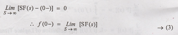
f(0-) indicates the value of f(t) just before t = 0 and f(0+) indicates the value of f(t) just after t = 0.

If function f(t) is continuous at t =0, then its value just before & just after t=0 will be same, (ie).

ƒ(0+) = f(0-) for f(t) continuous at t = 0. Substituting (4)^th equation in equation (3), we get.

This value is used to determine the initial value of ƒ (t) & its derivative

Hence proved

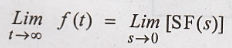
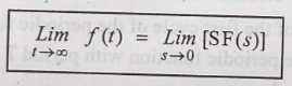
Final Value Theorem

If L[f(t)] = F(s), then the final value of f(t) is given as,

To Prove:

Proof :

We know that,

Let the limit for the above equation be considered as 'S' tends to zero, (ie).,

Consider LHS of the above equation (ie).,

comparing equation (1) & (2), we have,

Hence Proved.

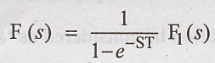
Laplace Transform of a Periodic Function

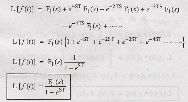
Let the Laplace transform of the first cycle of the periodic function be F₁(s). Then the lapalce transform of the periodic function with period T is given as,

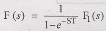
Thus the Laplace Transform of first cycle is multiplied by  to get Laplace trans of the periodic signal.

To Prove:

Proof :

Consider the following sine wave and its various cycles.

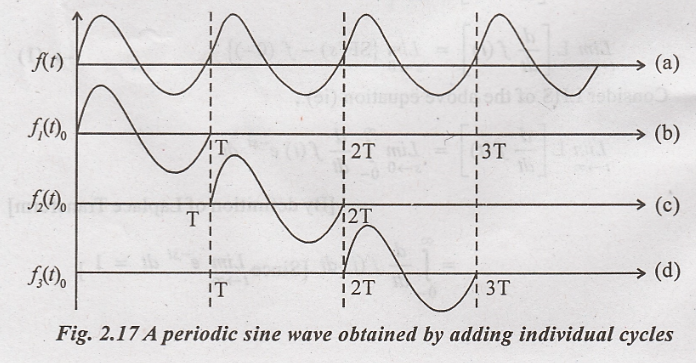
From the fig. 2.17, the complete sine wave (periodic) can be constructed by adding individual cycles of Figure 1.b, 1.c & 1.d and so. on.

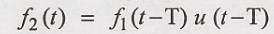
The signal f₂(t) is same as f₁(t), only it is shifted by 'T' with respect to f₁(t).

Here u(t-T) = 1 for t ≥ T. It shows that the equation is valid only for t ≥ T.

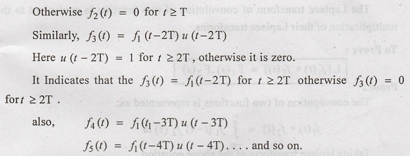
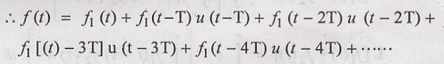
The periodic function can be obtained by adding infinite number of shifted first cycles

The Laplace transform of f₁(t) is F₁(s) and by applying the shifting property, we get,

Hence Proved

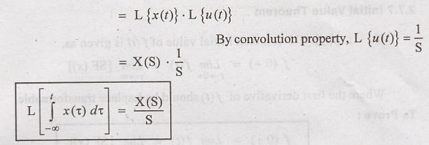
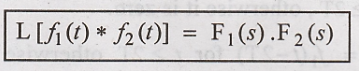
Convolution Theorem

The convolution theorem of Laplace transform states that,

If F₁(s) is laplace transform of f₁(t) and F₂(s) is the laplace transform of f₂(t) then,

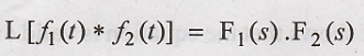
The Laplace transform of convolution of two function is equivalent to the multiplication of their Laplace transforms.

To Prove:

Proof:

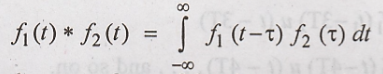
The convopution of two functions is represented as,

Taking laplace transform of the above equation,

Hence Proved

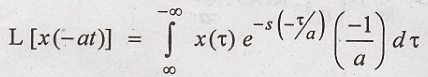
Time Scaling

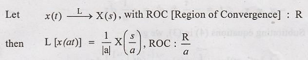
To Prove:

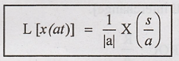
(ie) Expansion in time domain is equivalent to Compression in frequency domain and vice versa.

Proof :

By definition of Laplace transform,

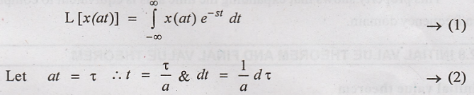
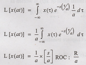
Integration Limits will remain the same, substituting equations (2) in (1), we get,

Let us now consider Negative value of a (ie) "- a”

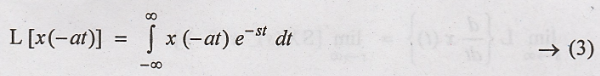
Let

Subtituting equations (4) in (3), we get,

[Here the Limits of Integration will interchange].

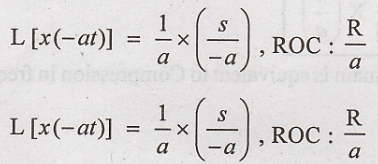
Hence Proved

This property shows that expanding the time axis is equivalent to compression in frequency domain.