Random Variable

RANDOM VARIABLE

A random variable is a rule that assigns a numerical value to each possible outcome of an experiment.

a. Discrete Random Variables, b. Continuous Random Variables

i. Random variable [A.U CBT Dec. 2009]

A real-valued function defined on the outcome of a probability experiment is called a random variable.

ii. Probability distribution function of X.

If X is a random variable, then the function F(x), defined by F(x) = P{X = x} is called the distribution function of X.

(a) (i) Discrete random variable

A random variable whose set of possible values is either finite or countably infinite is called discrete random variable.

Example

1. Let X represent the sum of the numbers on the 2 dice, when two dice are thrown. In this case the random variable X takes the values 2, 3, 4, 5, 6, 7, 8, 9, 10, 11 and 12. So X is a discrete random variable.

2. Number of transmitted bits received in error.

(ii) Probability mass function   

If X is a discrete random variable, then the function P (x) = P[X=x] is called the probability mass function of X.

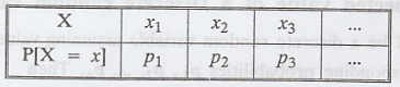
(iii) Probability distribution.

The values assumed by the random variable X presented with corresponding probabilities is known as the probability distribution of X.

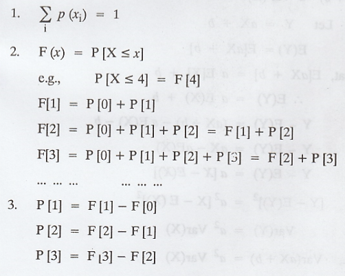
(iv) Cumulative distribution or Distribution function floss of X [for discrete R.V]

The cumulative distribution function F(x) of a discrete random variable X with probability distribution P (x) is given by

F(x) = P(X = x) =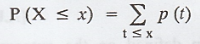 

x = -∞,... -2, -1, 0, 1, 2, ... ∞.

(v) Properties of distribution function

1. F(-∞) = 0

2. F(∞) = 1

3. 0 ≤ F(x) ≤ 1

4. F(x₁) ≤ F(x₂) if x₁ < x₂

5. P(x₁ < X ≤ x₂) = F(x₂) - F(x₁)

6. P(x₁ ≤ X ≤ x₂) = F(x₂) - F(x₁) + P[X = x₁]

7. P(x₁ < X < x₂) = F(x₂) - F(x₁) - P[X = x₂]

8. P(x₁ ≤ X < x₂) = F(x₂) - F(x₁) - P(X = x₂) + P(X = x1)

(vi) Results.

1. P(X ≤ ∞) = 1

2. P(X ≤ -∞) = 0

3. If x₁ ≤ x₂ then P (X = x₁) ≤ P(X = x₂)

4. P(X > x) = 1 - P[X ≤ x]

5. P(X ≤ x) = 1 - P(X > x)

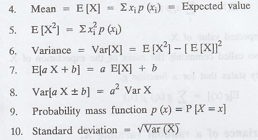
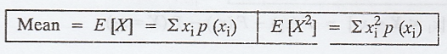
(vii) Expected value of a Discrete random variable X

Let X be a discrete random variable assuming values x₁, x₂, ..., x_n with corresponding probabilities p₁, p₂, ..., p_n. Then

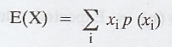
is called the Expected value of X.

E(X) is also called commonly the mean or the expectation of X.

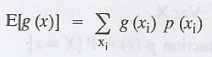
A useful identity states that for a function g,

(viii) The variance of a random varaible X.

It is defined by Var(X) = E[X - E (X)]²

The variance, which is equal to the expected value of the square of the difference between X and its expected value. It is a measure of the spread of the possible values of X.

A useful identity is that

Var(X) = E[X²]-[E(X)]²

The quantity  is called the standard deviation of X.

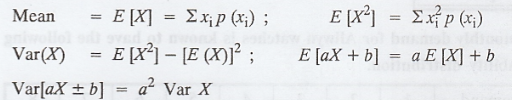
FORMULA

Note :

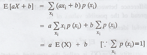
1. Prove that E[aX + b] = a E(X) + b.

Proof :

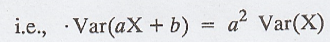
2. If X is a random variable then show that

Var(ax + b) = a² Var (X)

Proof :

Let Y = aX + b

E(Y) = E[aX + b]

We know that,

 

3. P[X = x_i] = p(x)

-> Probability function (or) Probability distribution (or) p.m.f (probability mass function)

4. f(x) -> p.d.f (probability density function) (or) density function.

5. F(x) -> c.d.f (cumulative distribution function) (or) distribution function.

Problems under the distribution function for discrete random variable

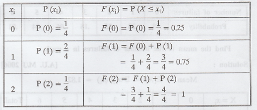
Example 1.4.1 ([Given P (xi) to find F (xi) type]

For the following probability distribution (i) Find the distribution function of X. (ii) What is the smallest value of x for which P(X ≤ x) > 0.5

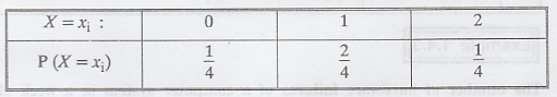
Solution :

(i)

(ii) The smallest value of x for which P (X ≤ x_i) > 0.5 is 1.

Note : The smallest value of x for which P (X ≤ x_i) > 0.1 is 0 and

The smallest value of x for which P (X ≤ x_i) > 0.8 is 2.

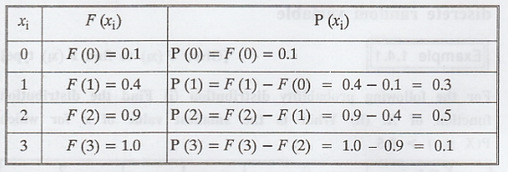
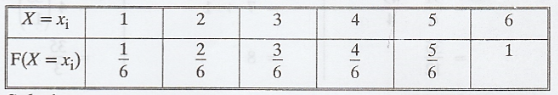
Example 1.4.2 [Given F (xi) to find P (xi) type]

Obtain the probability function (or) probability distribution from the following distribution function.

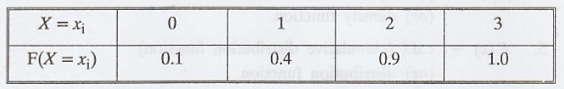
Solution :

To Find P(x_i)

Example 1.4.3

The number of hardware failures of a computer system in a week of operations has the following pmf:

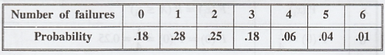
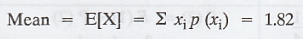
Find the mean of the number of failures in a week. [A.U. M/J 2006]

Solution :

Example 1.4.4

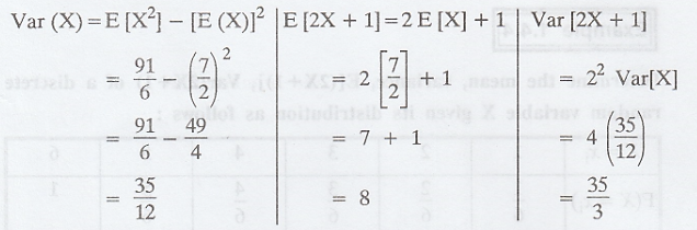
Determine the mean, variance, E[(2X+1)], Var(2X+1) of a discrete random variable X given its distribution as follows :

Solution :

Example 1.4.5

The monthly demand for Allwyn watches is known to have the following probability distribution.

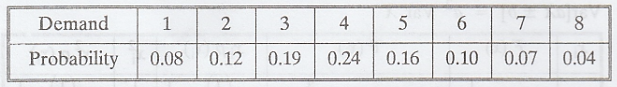
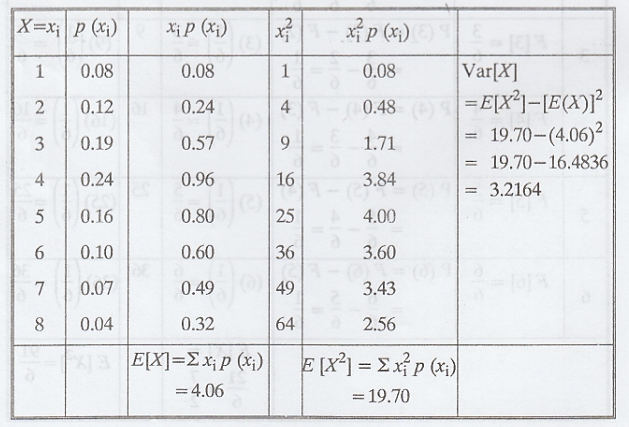
Determine the expected demand for watches. Also compute the variance. [A.U. N/D 2006]

Solution:

Let X denote the demand

Example 1.4.6

When a die is thrown, X denotes the number that turns up. Find E (X), E (X²) and var (X). [A.U. M/J 2006, A.U N/D 2019 (R17) PS]

Solution :

X is a discrete random variable taking values, 1, 2, 3, 4, 5, 6 and with probability 1/6 for each

Example 1.4.7

Determine the constant K given the following probability distribution of discrete random variable X. Also find mean and Variance of X.

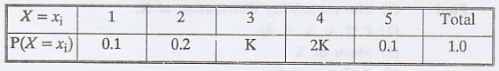
Solution:

We know that,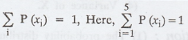 

we have, 0.1 + 0.2 + K + 2K + 0.1 = 1

i.e., 3K = 1 - 0.4 = 0.6

K = 0.2

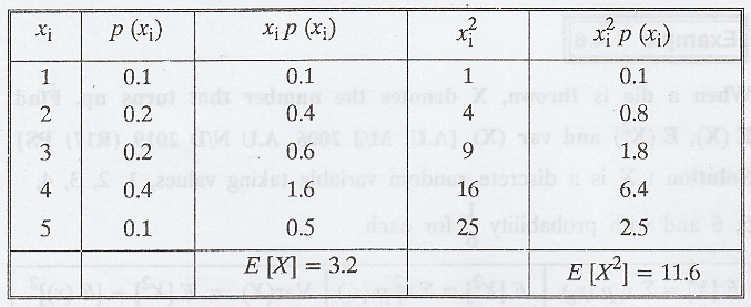
Var[X] = E[X²] - [E(X)]² = 11.6 - (3.2)2 = 11.6 - 10.24 = 1.36

Example 1.4.8

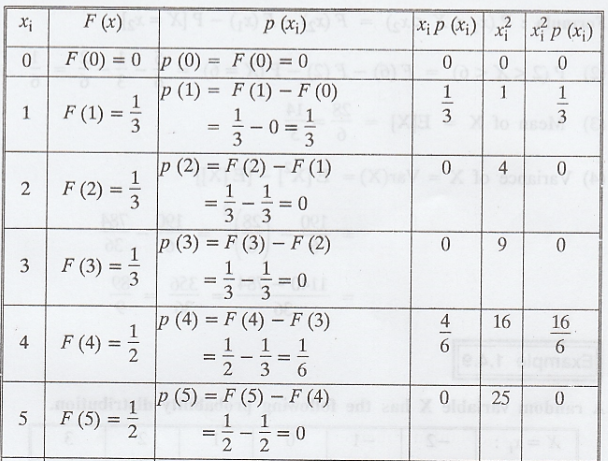
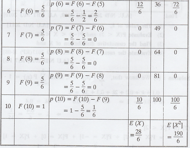
If X has the distribution function

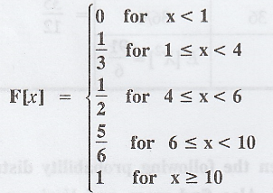
Find (1) The probability distribution of X.

(2) P (2 < X < 6)

(3) Mean of X

(4) Variance of X. [A.U. A/M. 2008]

Solution:

(1) The probability distribution of X.

 

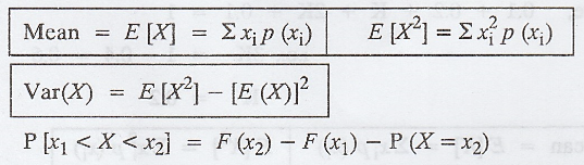
Formula:

(1) P(x₁ < x < x₂) = F(x₂) - F(x₁) - P[X = x₂]

(2) P(2 < X < 6) = F(6) - F(2) - P(X = 6) =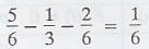 

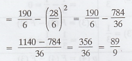
(3) Mean of X = E[X] = 28/6 = 14/3

(4) Variance of X = Var(X) = E[X²] - [E[X]]² =

Example 1.4.9

A random variable X has the following probability distribution.

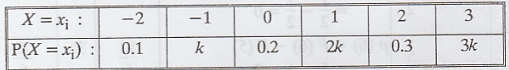
Find

(1) The value of k,

(2) Evaluate P(X < 2) and P(-2 < X < 2)

(3) Find the cumulative distribution of X and

(4) Evaluate the mean of X. [A.U. N/D 2017 (RP) R-08] [A.U N/D 2018, R17 PS] [A.U. N/D 2007, M/J 2009, A.U CBT M/J 2010] [A.U N/D 2011]

Solution:

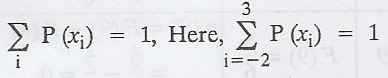
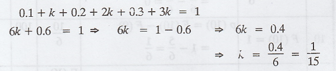
(1) We know that,

(2) (i) P[X < 2] = P[X = -2] + P[X -1]+ P[X = 0] + P[X = 1]

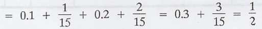
(ii) P [-2 < x < 2]

= P[X = -1] + P[X = 0] + P[X = 1]

=  1/15 + 0.2 + 2/15 = 0.2 + 3/15 = 2/5

(3)

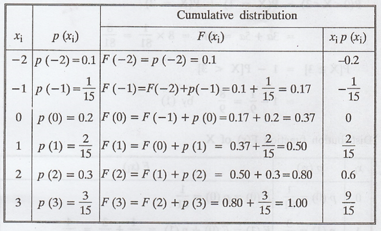
(4) Mean = E[X] =  = 16/15

Example 1.4.10

A discrete random variable X has the following probability distribution.

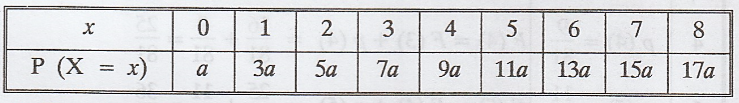
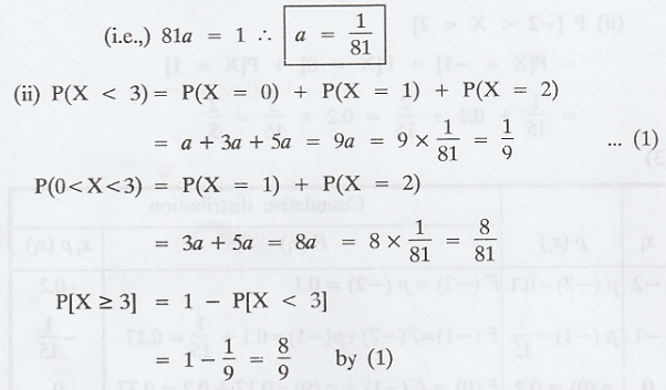
(i) Find the value of a. [A.U CBT N/D 2011, Trichy M/J 2011] [AU Tvli. A/M 2009]

(ii) Find P(X < 3), P(0 < x < 3), P(X ≥ 3)

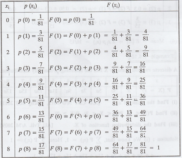
(iii) Find the distribution function of X.

Solution:

(i) We know that, 

a + 3a + 5a + 7a + 11a + 13a + 15a + 17a = 1

Distribution function F(x) of X.

Example 1.4.11

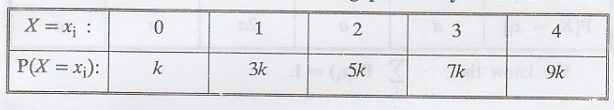
A random variable X has the following probability function :

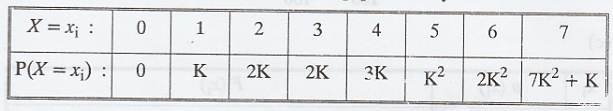
(a) Find K

(b) Evaluate P[X < 6], P[X ≥ 6]

(c) If P[X ≤ C] > 1/2, then find the minimum value of C.

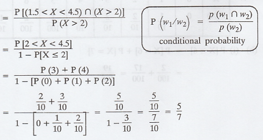
(d) Evaluate P [1.5 < X< 4.5/X > 2]

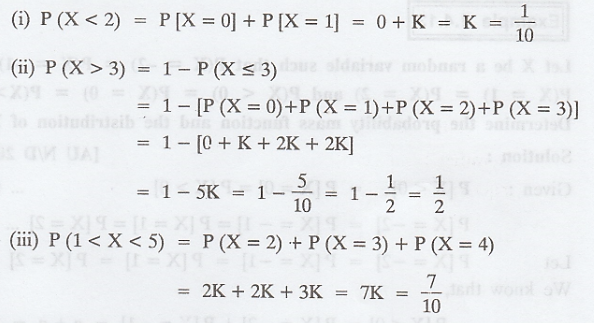
(e) Find P [X < 2], P[X > 3], P[1 < X < 5] [A.U N/D 2010, M/J 2012, M//J 2014 [A.U A/M 2015 R-] [A.U M/J 2007, N/D 2008] [A.U. Tvli A/M 2009]

Solution:

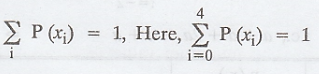
(a) We know that, 

i.e., 0 + K + 2K + 2K + 3K + K2 + 2K2 + 7K2 + K = 1

i.e., 10 K2 + 9K - 1 = 0

=> K = -1 or K = 1/10

Since, P(X) ≥ 0 the value K = -1 is not permissible

Hence, we have K = 1/10

(b) (i) P[X ≥ 6] = P [X = 6] + P[X = 7]

= 2/100 + 17/100 = 19/100

(ii) P [X < 6] = 1 - P[X ≥ 6]

= 1 - 19/100 = 81/100

(c)

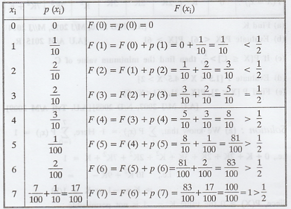
The minimum value of C = 4. ['.' P[X ≤ C] > 1/2]

(d) P [1.5 < X < 4.5/X > 2]

(e) 

Example 1.4.12

A random variable 'X' has the following probability function :

Find k, P [X ≥ 3] and P (0 < x < 4) [A.U. Tvli. A/M 2009]

Solution:

(i) We know that, 

 

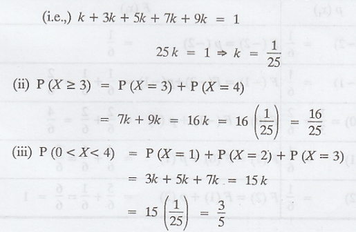
Example 1.4.13

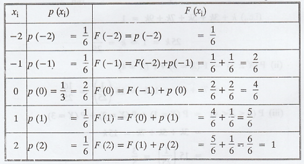
Let X be a random variable such that P(X = -2) = P(X = -1) = P(X = 1) = P(X = 2) and P(X < 0) = P(X = 0) = P(X > 0). Determine the probability mass function and the distribution of X. [AU N/D 2006]

Solution :

Given:

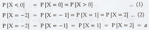
We know that,

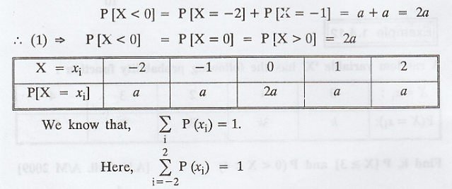
i.e., a + a + 2a + a + a = 1 => a = 1 => a = 1/6

 

Example 1.4.14

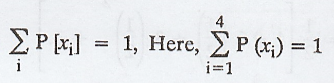
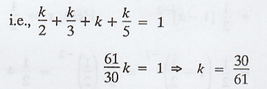
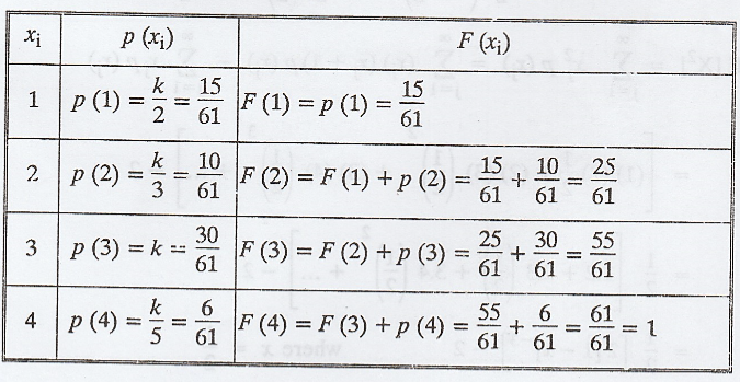
If the random variable X takes the values 1, 2, 3 and 4 such that 2P(X = 1) = 3P(X = 2) = P(X = 3) = 5P(X = 4) find the probability distribution and cumulative distribution function of X.

[A.U CBT A/M 2011, A.U N/D 2012, A.U A/M 2017 R8] [IIOS QM U.A [A.U A/M 2019 (R13) PQT] [A.U A/M 2015 (RP) R8]

Solution :

X is a discrete random variable.

Given: 2P[X = 1] = 3P[X = 2] = P[X = 3] = 5P[X = 4]

Let 2P[X = 1] = 3P[X = 2] = P[X = 3] = 5P[X = 4] = k ...........(1)

We know that, 

Example 1.4.15

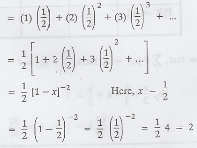
The probability function of an infinite discrete distribution is given by P[X = j] = 1/2^j, j = 1, 2, ..., ∞. Find the mean and variance of the distribution. Also find P[X is even], P [X ≥ 5] and P[X is divisible by 3]. [A.U. N/D 2006] [A.U N/D 2011]

Solution: Given: P[X = j] = 1/2^j = (1/2)^j

Mean = E[X] = 

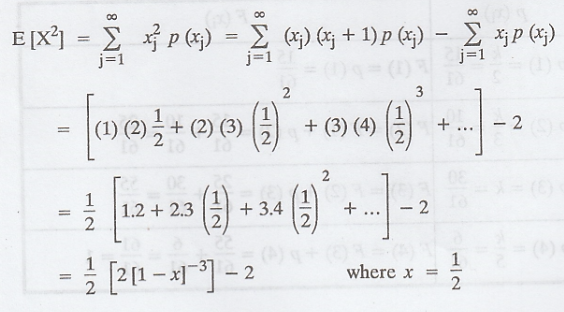
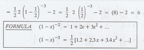
Variance of X = Var(X) = E[X²] - [E[X]]² = 6 - (2)² = 6 - 4 = 2

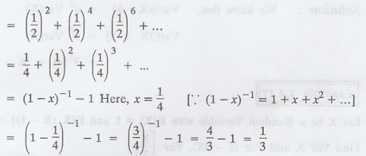
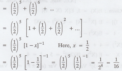
(1) P[X is even] = P[X = 2] + P[X = 4] + .....

(2) P [X ≤ 5] = P[X = 5] + P [X = 6] + ...

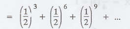
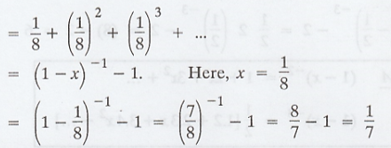
(3) P[X is divisible by 3] (or) P[X is multiple of 3]

= P[X = 3] + P[X = 6] + ...

 

Example 1.4.16

If Var(X) = 4, then find Var(3X + 8), where X is a random variable. [A.U, Model] [A.U Tvli M/J 2011]

Solution:

We know that, Var(aX + b) = a² Var(X)

Var(3X + 8) = 3² Var(X) = 3²[4] = 36

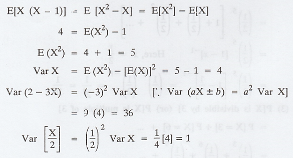
Example 1.4.17

Let X be a Random Variable with E(X) = 1 and E[X (X - 1)] = 4. Find Var X and Var (2 - 3X), Var [X/2] [A.U. May, 2000], [A.U. A/M. 2008]

Solution :

Example 1.4.18.

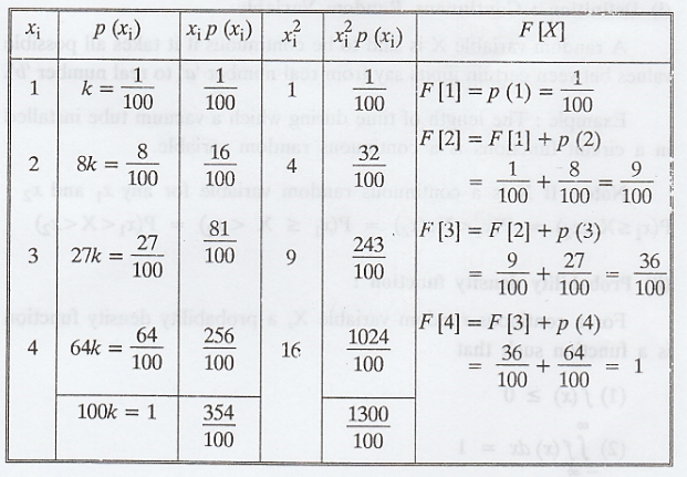
If the probability mass function of a r.v. X is given by P(X = r) = kr³, r = 1, 2, 3, 4 find

(i) the value of k,

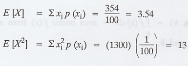
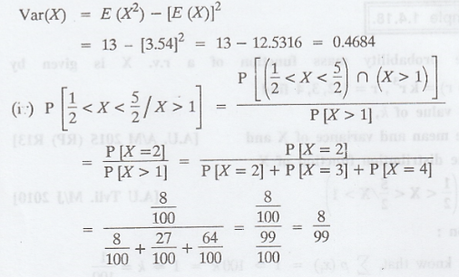
(ii) the mean and variance of X and [A.U. A/M 2015 (RP) R13]

(iii) the distribution function of X

(iv) P (1/2 < X < 5/2 / X > 1) [A.U Tvli. M/J 2010]

Solution :

(i) We know that,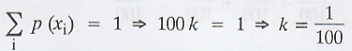 

(ii) & (iii) Given: P(X = r) = kr³, r = 1, 2, 3, 4