Normal Distribution

NORMAL DISTRIBUTIONS

The Normal Distribution was introduced by the French Mathematician Abraham De Moivre in 1733. Demoivre, who used this distribution to approximate probabilities connected with coin tossing, called if the exponential bell-shaped curve.

i. Normal Distribution

A normal distribution is a continuous distribution given by 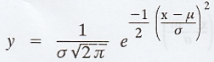 where X is a continuous normal variate distributed with density function f(x) =  with mean µ and standard deviation σ.

ii. Deviation of the distribution

Let the equation of the normal curve be y = 

It will be a normal probability curve if

In the above derivation, mean has been taken at the origin, but if however another point is taken as the origin such that the excess of the mean over the arbitrary origin is 'm', then

 is the standard form of the normal curve with origin at (m, 0).

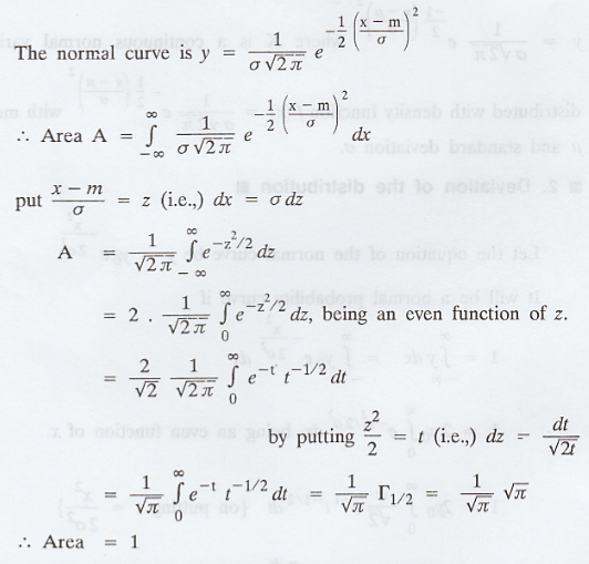
iii. Area under the normal curve is unity

The normal curve is y =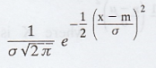 

iv. Characteristics of the Normal Distribution

The diagram of a normal distribution is given below. It is called normal curve. It suggests several important properties of the normal distribution.

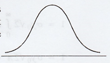
a. The normal distribution is a symmetrical distribution and the graph of the normal distribution is bell shaped.

b. The curve has a single peak point (i.e.,) the distribution is unimodal.

c. The mean of the normal distribution lies at the centre of normal curve.

d. Because of the symmetry of the normal curve, the median and mode are also at the centre of the normal curve. Hence in a normal distribution the mean, median and mode coincide.

e. The tails of the normal distribution extend indefinitely and never touch the horizontal axes. That is, we say that the normal curve approaches asymptotically on either side of its horizontal axes.

f. The normal distribution is a two parameter probability distribution. The parameters mean and standard deviation (µ, σ) completely determine the distribution.

g. Area property: In a normal distrbution, about 67% of the observations will lie between mean ± S.D (i.e., µ ± σ). About 95% of the observations will lie between mean ± 2 S.D (µ ± 2 σ). About 99% of the observations will lie between mean ± 3 S.D (i.e., µ ± 3 σ).

v. Standard normal probability distribution

If X is a normally distributed random variable µ and s are respectively its mean and standard deviation, then Z = (X - µ)/ σ is called standard normal random variable.

Special table called table of areas under normal curve is available to determine probabilities that the random variable lies in a given range of values of the variables. Using the table, we can determine the probability for X, taking a value less than x (X < x) and also for a given probability we determine the value x such that X < x.

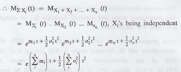
vi. The additive property of Normal Distribution

If X₁, X₂, ... X_n are independent normal variates with parameters (m₁, σ₁), (m₂, σ₂) ... (m_n, σ_n) respectively, then X₁ + X₂ + ... + X_n is also a normal variate with parameter (m, σ),

where m = m₁ + m₂ + ... + m_n and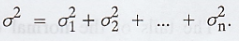 

Proof : 

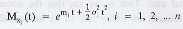
which is the moment generating function of a normal variate with mean  and variance 

Hence, X₁ + X₂ + ... + X_n follow normal distribution with mean  and variance 

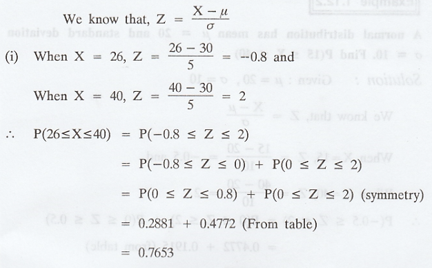
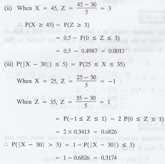
Example 1.12.1

X is a normal variate with mean 30 and S.D 5. Find the probabilities that (i) 26 ≤ X ≤ 40, (ii) X ≥ 45, (iii) |X - 30| > 5 [A.U Tvli A/M 2009]

Solution

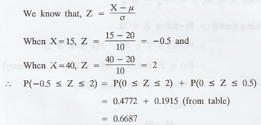
Example 1.12.2

A normal distribution has mean µ = 20 and standard deviation σ = 10. Find P(15 ≤ X ≤ 40)

Solution :

Given: µ = 20, σ = 10

Example 1.12.3

The average seasonal rainfall in a place in 16 inches with a S.D. of 4 inches. What is the probability that in a year the rainfall in that place will be between 20 and 24 inches ?

Solution :

Example 1.12.4

If X is a random variable normally distributed with mean zero and variance σ², find E [|X|].

Solution:

E [|X|] = Mean deviation about origin

= Mean deviation about mean (.'. mean = 0)

Mean deviation about mean = 4σ/5

.'. E [|X|] = 4σ/5.

Example 1.12.5

X is a normal variate with mean 1 and variance 4. Y is another normal variate independent of X with mean 2 and variance 3. What is the distribution of X + 2Y.

Solution:

Since X and Y are independent normal variates, X + 2Y will also be a normal variate by the addition property and

Mean of (X + 2Y) = = E(X + 2Y) = E(X) + 2E(Y)

= 1 + 2 x 2 = 5 [.'. E(X) = 1, E(Y) = 2]

Variance of (X + 2Y) = V(X + 2Y) = V(X) + 4V(Y) ['.' X and Y are independent]

= 4 + 4 x 3 = 16 [V(X) = 4, V(Y) = 3]

.'. X + 2Y will follow normal with mean 5 and variance 16.

Example 1.12.6

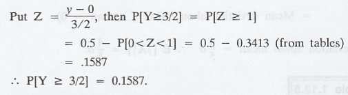
If X is normal with mean 2 and standard deviation 3, describe the distribution of Y = 1/2 (X - 1) find P[Y ≥ 3/2]

Solution :

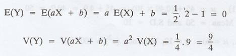
Given X follows normal with mean 2 and variance 9. The distribution of Y = aX + b is also normal with

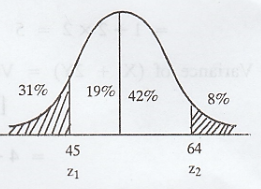
Example 1.12.7

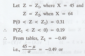
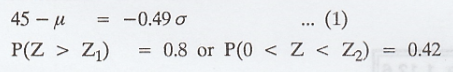
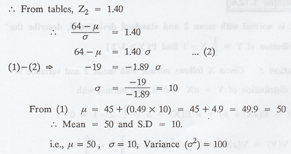
In a normal distribution, 31% of the items are under 45 and 8% are over 64. Find the mean and variance of the distribution. [A.U N/D 2015 R13, RP] [A.U A/M 2019 (R13) RP] [A.U CBT N/D 2011] [A.U M/J 2012]

Solution:

We know that, Z = 

Example 1.12.8

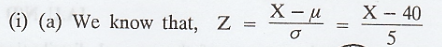
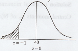
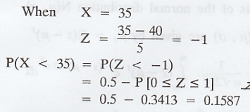
(i) A company finds that the time taken by one of its engineers to complete or repair job has a normal distribution with mean 40 minutes and standard deviation 5 minutes. State what proportion of jobs take: (a) less than 35 minutes (b) more than 48 minutes

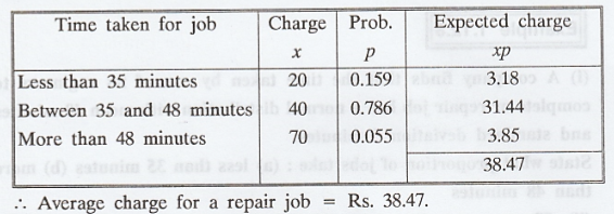
(ii) The company charges Rs. 20 if the job takes less than 35 minutes, Rs. 40 if it takes between 35 and 48 minutes and Rs. 70 if it takes more than 48 minutes. Find the average charge for a repair job.

Solution :

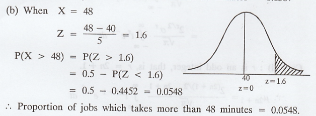
.'. Proportion of jobs which takes more than 48 minutes = 0.0548.

(ii) P(35 < X < 48) = P( -1 < Z < 1.6)

= P(-1 < Z < 0) + P(0 < Z < 1.6)

= 0.3413 + 0.4452 = 0.7865

.'. Proportion of jobs which takes between 35 and 48 minutes = 0.786.

Example 1.12.9

Find the nth central moments of normal distribution. [AU M/J 2007] [A.U N/D 2014 (RP) R-8]

Solution:

Central moments of the normal distribution N(µ, σ)

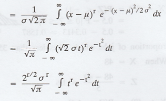
Central moments µ_r of N(µ, σ) are given by µ_r = E(x - µ)^r

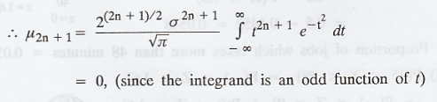
Case (i) r is an odd integer, that is, r = 2n + 1.

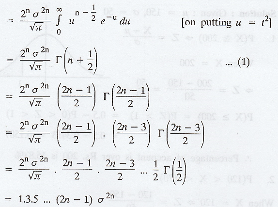
Case (ii) r is an even integer, that is r = 2n

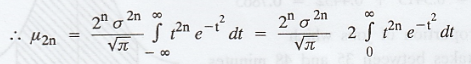
['.' the integrand is an even function of t]

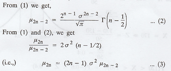
(3) gives a recurrence relation for the even order central moments of the normal distribution N (µ, σ).

Example 1.12.10

The savings bank account of a customer showed an average balance of Rs. 150 and a standard deviation of Rs. 50. Assuming that the account balances are normally distributed.

1. What percentage of account is over Rs. 200 ?

2. What percentage of account is between Rs. 120 and Rs. 170? [AU N/D 2006]

3. What percentage of account is less than Rs. 75 ?

Solution

Given: µ = 150, σ = 50

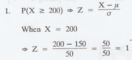
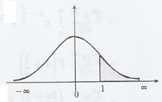
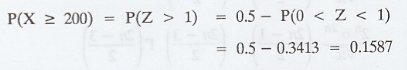
.'. Percentage of account is over Rs. 200 is 15.87%

2. P(120 < x < 170)

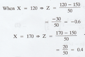
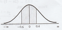
.'. Percentage of account is between Rs. 120 and Rs. 170 is 38.11%

3. P(X < 75) => Z = 

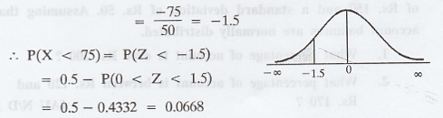
.'. Percentage of account is less than Rs. 75 is 6.68%

Example 1.12.11

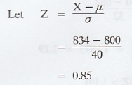
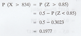
An electrical firm manufactures light bulbs that have a life, before burn-out, that is normally distributed with mean equal to 800 hours and a standard deviation of 40 hours. Find

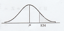
(1) the probability that a bulb burns more than 834 hours

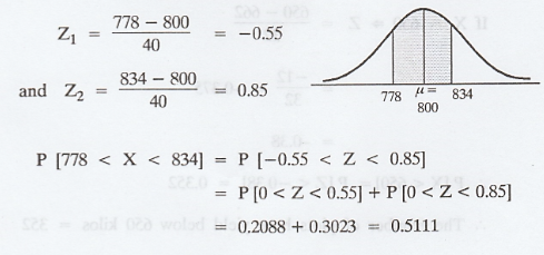
(2) the probability that bulb burns between 778 and 834 hours. [AU N/D 2006] [A.U N/D 2018 R-13 PQT]

Solution

(1) Given: µ = 800 hours σ = 40 hours

(2) Given: X₁ = 778 and X₂ = 834

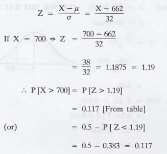
Example 1.12.12

The mean yield for one-acre plot is 662 kilos with standard deviation 32 kilos. Assuming normal distribution, how many one-acre plots in a patch of 1,000 plots would you expect to have yield over 700 kilos, below 650 kilos. [AU A/M 2008]

Solution:

Given: µ = 662, σ = 32

Standard normal variate

.'. The number of plots have yield over 700 kilos = 117

.'. The number of plots have yield below 700 kilos = 117

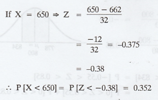
.'. The number of plots have yield below 650 kilos = 352

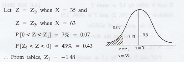
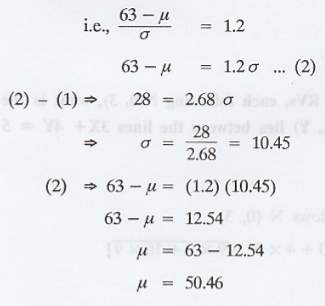
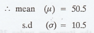
Example 1.12.13

In a distribution exactly normal 7% of the items are under 35 and 89% are under 63. What are the mean and standard deviation of the distribution? [AU Nov. 2005]

Solution:

We know that, Z = X - µ / σ

Example 1.12.14

The independent RVS X and Y have distributions N(45, 2) and N(44, 1.5) respectively. What is the probability that randomly chosen values of X and Y differ by 1.5 or more? [A.U N/D 2011]

Solution:

X is N (45, 2) and Y is N(44, 1.5)

.'. By the property of additive

U = X - Y follows the distribution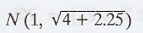 

i.e., N (1, 2.5)

P[X and Y differ by 1.5 or more]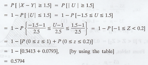

Example 1.12.15

If X and Y are independent RVs, each following N(0, 3), what is the probability that the point (X, Y) lies between the lines 3X + 4Y = 5

and 3X + 4Y = 10?

Solution :

X follows N(0, 3) and Y follows N (0, 3).

U = 3X + 4Y follows 

i.e., N(0, 15)

P[the point (X, Y) lies between the lines 3X + 4Y = 5 and 3X + 4Y = 10]

= P [5 < 3X + 4Y < 10]

= P [5 < U < 10]

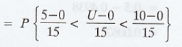
= P [0.33 < Z < 0.67]

where Z is the standard normal variable

= P(0 < Z < 0.67) - P (0 < Z < 0.33)

= 0.2486 - 0.1293, by using the table

= 0.1193

Example 1.12.16

The peak temperature T, as measured in degrees Fahrenheit, on a particular day is the Gaussian (85, 10) random variable. What is P (T > 100), P (T < 60) and P [70 ≤ T ≤ 100]? [A.U A/M. 2015, R13]

Solution :

Given µ = 85, σ = 10

We know that, Z = T - µ / σ

(ii) When T = 60, Z = 60 - 85 / 10 = -2.5

P[T < 60] = P[Z < -2.5]

= 0.5 - P[0 ≤ Z ≤ 2.5]

= 0.5 - 0.4938

= 0.0062

(iii) When T = 70, Z = 70 - 85 / 10

P [70 = T = 100] = P[-1.5 ≤ Z ≤ 1.5]

= P[-1.5 = Z = 0] + P [0 = Z = 1.5]

= 0.4332 + 0.4332 = 0.8664

EXERCISE 1.12

1. If  is the moment generating function of a normal random variable X, find P [-1 < X < 9].

2. If f(x) =  is the density function of a normal distribution, k being a constant, find the mean and standard deviation of the distribution. [Ans. Mean = 2/3; standard deviation = 1/3v2

3. If X is normally distributed with mean zero and variance unity, what is the expectation and variance of e^aX? [Ans.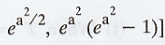 

4. The quartiles of a normal distribution are 8 and 14 respectively. Estimate the mean and standard deviation. [Ans. µ = 11, σ = 4.4]

5. Given that X is distributed normally. P [X ≤ 45] = 0.31 and P [X ≥ 64] = 0.08, find the mean and standard deviation of the distribution. [Ans. m = 50, σ² = 100]

6. In a sample of 1000 cases, the mean of a certain test is 14 and standard deviation is 2.5. Assuming the distribution to be normal find (i) How many students score between 12 and 15 ? (ii) How many score above 18 ? (iii) How many score below 18 ? (iv) How many score 16? [Ans. (i) 443, (ii) 54, (iii) 8, (iv) 116]

7. The average test marks in a particular class is 79. The S.D is 5. If the marks are distributed normally, how many students in a class of 200 did not receive marks between 75 and 82? [Ans. 97]

8. In a sample of 120 workers in a factory the mean and standard deviation of wages were Rs. 11.35 and Rs. 3.03 respectively. Find the percentage of workers getting wages between Rs. 9 and Rs. 17 in the whole factory assuming that the wages are normally ICI distributed? [Ans. 75.09%]

9. At a certain examination 10% of the students who appeared for the paper in statistics got less than 30 marks and 97% of the students got less than 62 marks. Assuming the distribution is normal, find the mean and the S.D. of the distribution.

[Ans. µ = 43.04, σ = 10.03]