Joint Distribution - Marginal and conditional distributions

Joint distributions - marginal and conditional distributions

i. Joint probability distribution

The probabilities of the two events A = {X ≤ x} and B = {Y ≤ y} defined as functions of x and y, respectively, are called probability distribution functions.

F_x (x) = P(X ≤ x);

_Fy (y) = P(Y ≤ y)

Note: We introduce a new concept to include the probability of the joint event {X ≤ x, Y ≤ y}.

ii. Joint probability distribution of two random variables X and Y

We define the probability of the joint event {X ≤ x, Y ≤ y}, which is a function of the numbers x and y, by a joint probability distribution function and denote it by the symbol F_{x, y} (x, y).

Hence F_X,Y (x,y) = p (X ≤ x, Y ≤ y}

Note: Subscripts are used to indicate the random variables in the bivariate probability distribution. Just as the probability mass function of a single random variable X is assumed to be zero at all values outside the range of X, so the joint probability mass function of X and Y is assumed to be zero at values for which a probability is not specified.

iii. Properties of the joint distribution.

A joint distribution function for two random variables X and Y has several properties.

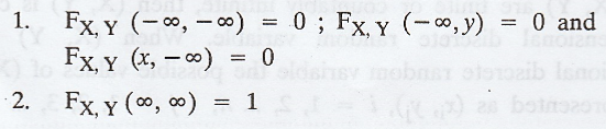
For a given function to be a valid joint distribution function of two dimensional RVs X and Y, it must satisfy the properties (1), (2) and (5)

iv. Joint probability function of the discrete random variables X and Y

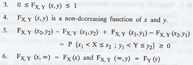
If (X, Y) is a two-dimensional discrete random variable such that f(x_i, y_j) P(X = x_i, Y = y_j) = P_ij is called the joint probability function or joint probability mass function of (X, Y) provided the following conditions are satisfied.

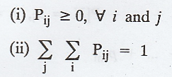
The set of triples {x_i, y_j, P_ij}, i = 1, 2, … n, j = 1, 2, ... m is called the joint probability distribution of (X, Y). It can be represented in the form of table as given below.

v. Marginal probability distribution

If more than one random variable is defined in a random experiment, it is important to distinguish between the joint probability distribution of X and Y and the probability distribution of each variable individually. The individual probability distribution of a random variable is referred to as its marginal probability distribution.

In general, the marginal probability distribution of X can be determined from the joint probability distribution of X and other random variables.

vi. Marginal probability mass function of X

If the joint probability distribution of two random variables X and Y is given, then the marginal probability function of X is given by

Note: The set {x1, P1.} is called the marginal distribution of X.

vii. Marginal Probability mass function of Y

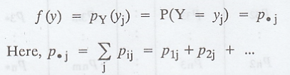
If the joint probability distribution of two random variables X and Y is given, then the marginal probability function of Y is given by

viii. Conditional Probability distribution

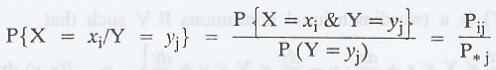 is called the conditional probability function of X, given Y = y_j

The collection of pairs 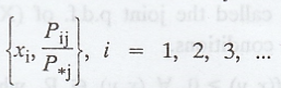 is called the conditional probability distribution of X, given Y = y_j

Similarly, the collection of pairs,  is called the conditional probability distribution of Y given X = x_i.

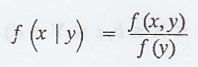
let (X, Y) be the two dimensional continuous R.V. The conditional probability density function of X given Y is denoted by f(x | y) and is defined as,

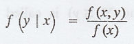
Similarly, the conditional probability density function of Y given X is denoted by f (y | x) and is defined as,

ix. Independent random variables

Two R.V's X and Y are said to be independent if f(x,y) = f(x). f(y) where f(x, y) is the joint probability density function of (X, Y), f(x) is the marginal density function of X and f(y) is the marginal density function of Y.

Also we can say, the random variables X and Y are said to be independent R.V's if

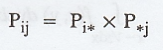
where Pij is the joint probability function of (X, Y), Pix is the marginal probability function of X and P*j is the marginal probability function of Y.

x. Joint probability density function

If (X, Y) is a two-dimensional continuous R.V such that

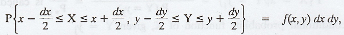
then f(x, y) is called the joint p.d.f. of (X, Y), provided f(x, y) satisfies the following conditions.

(i) f(x, y) ≥ 0, V (x,y) ε R, where 'R' is the range space.

 

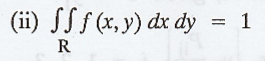
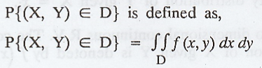
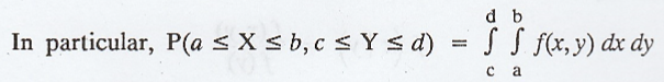
Moreover, if D is a subspace of the range space R,

xi. Cumulative distribution function

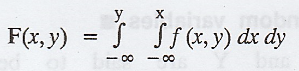
If (X, Y) is a two-dimensional continuous random variable, then F(x,y) = P(X ≤ X and Y ≤ y) is called the cdf of (X, Y) and is defined as,

xii. Marginál density function [A.U CBT Dec. 2009]

If (X, Y) is a two-dimensional continuous random variable, then

Let (X, Y) be the two dimensional random variable. Then, the marginal probability density function of X is denoted by f(x) and is defined as,

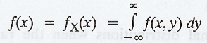
Similarly, the marginal probability density function of Y is denoted by f(y) and is defined as,

xiii. Joint probability density function

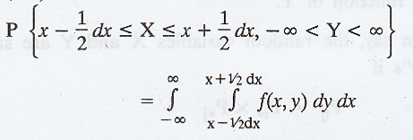
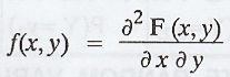
Let (X, Y) be the two dimensional random variable and F(x, y) be the joint probability distribution function. Then the joint probability density function of X and Y is denoted by f(x, y) and is defined as,

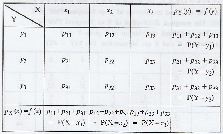
xiv.Table - I

To calculate marginal distributions when the random variable X takes horizontal values and Y takes vertical values.

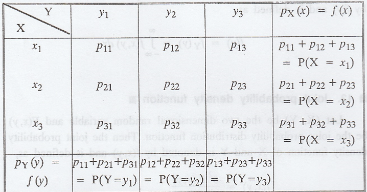
xv. Table - II

To calculate marginal distributions when the random variable X takes vertically and Y takes horizontally.

PROBLEMS UNDER DISCRETE RANDOM VARIABLES :

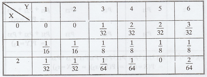
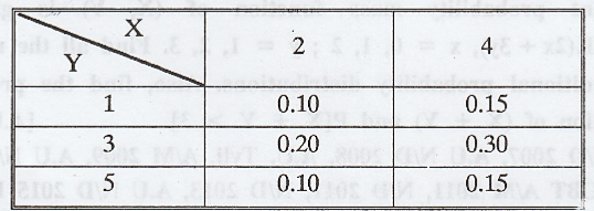
Example 2.1.1

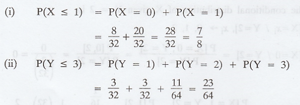
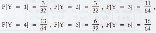
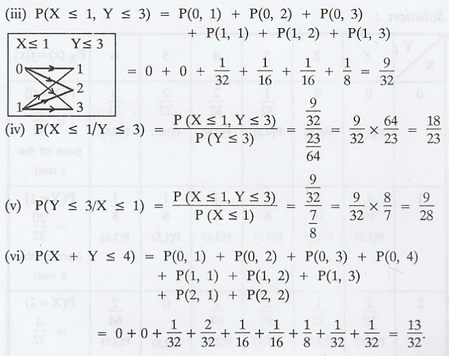
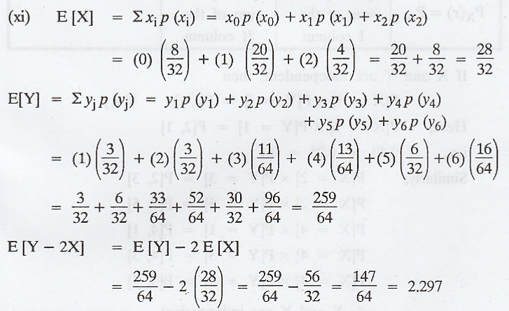
From, the following table for bivariate distribution of (X, Y) find (i) P(X ≤ 1), (ii) P(Y ≤ 3), (iii) P(X ≤ 1, Y ≤ 3), (iv) P(X ≤ 1 / Y ≤ 3), (v) P (Y ≤ 3 / X ≤ 1), (vi) P (X + Y ≤ 4). (vii) The marginal distribution of X or Marginal PMF of X (viii) The marginal distribution of Y or Marginal PMF of Y (ix) The conditional distribution of X given Y = 2 (x) Examine X and Y are independent. (xi) E[Y – 2X]

Solution :

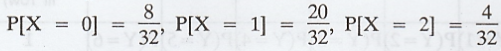
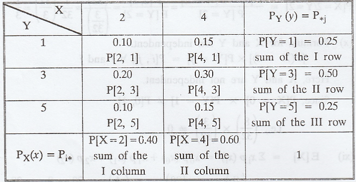
(vii) The marginal distribution of X is

(viii) The marginal distribution of Y is

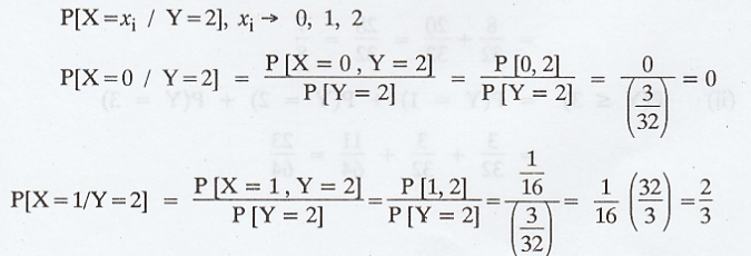
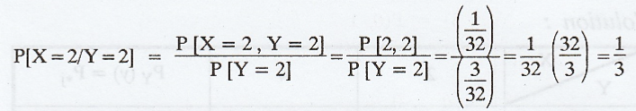
(ix) The conditional distribution of X given Y = 2 is

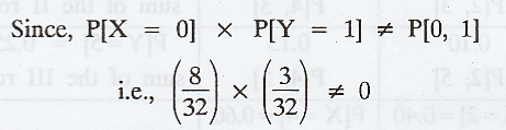
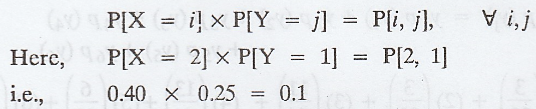
(x) Formula for X and Y are independent.

Here, X and Y are not independent.

Example 2.1.2

Let X and Y have the following joint probability distribution.

Show that X and Y are independent.

Solution :

If X and Y are independent, then

Similarly, 

.'. X and Y are independent.

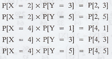
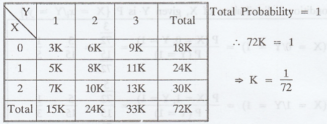
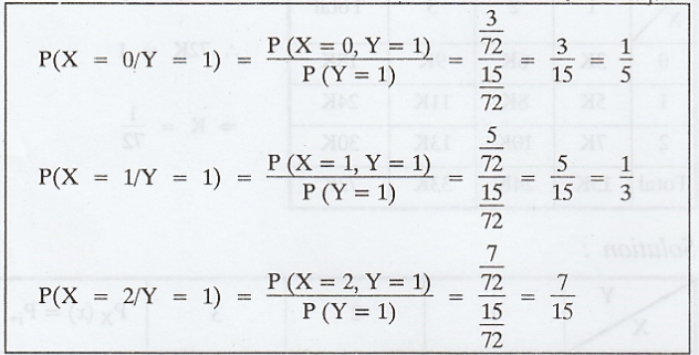
Example 2.1.3

The joint probability mass function of (X, Y) is given by P(x, y) = K(2x + 3y), x = 0, 1, 2; y = 1, 2, 3. Find all the marginal and conditional probability distributions. Also, find the probability distribution of (X + Y) and P[X + Y > 3]. [A.U. 2004] [A.U N/D 2007, A.U N/D 2008, A.U. Tvli. A/M 2009, A.U N/D 2014] [A.U CBT A/M 2011, N/D 2011, N/D 2013, A.U N/D 2015 R13 RP] [A.U A/M 2017 R-13] [A.U N/D 2018 (R17) PS]

Solution :

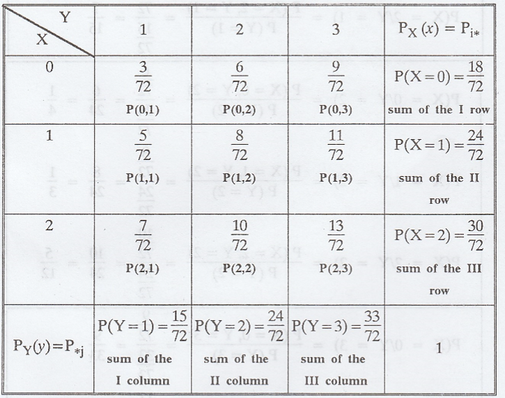
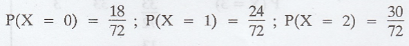
The marginal distribution of X :

The marginal distribution of Y :

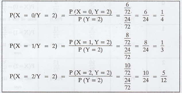
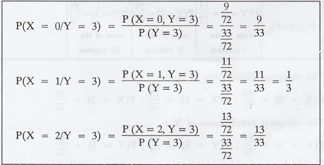
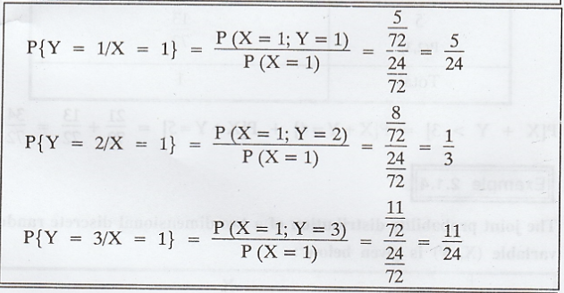
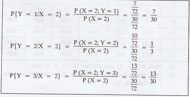
The conditional distribution of X, given Y is P {X = x_i/Y = y_j}

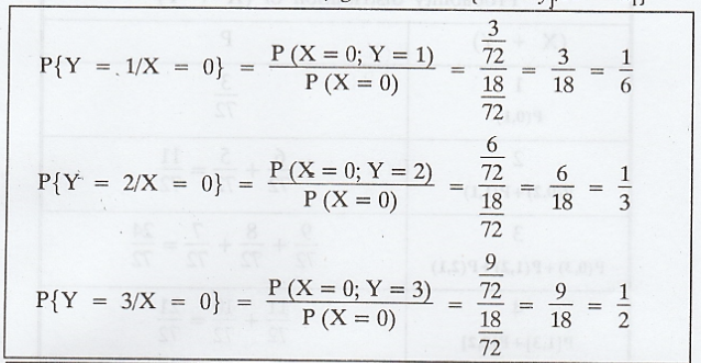
The conditional distribution of Y, given X is P {Y = y_j/X = x_i}

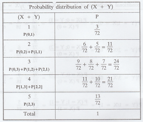
P[X + Y > 3] = P[X + Y = 5] = 21/72 + 13/72 = 34/72

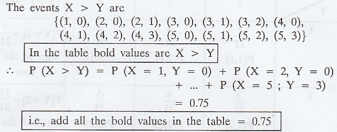
Example 2.1.4

The joint probability distribution of a two-dimensional discrete random variable (X,Y) is given below :

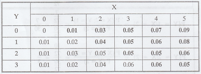
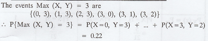
(i) Find, P(X > Y) and P{Max (X, Y)

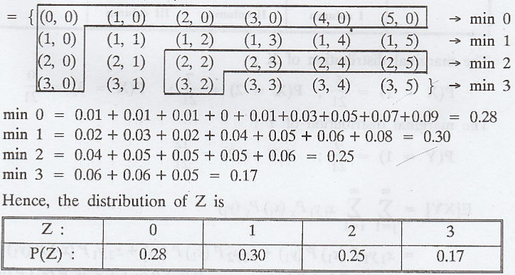
(ii) Find, the probability distribution of the random variable, Z = min (X,Y)

Solution :

Given Z = min (X,Y)

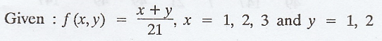
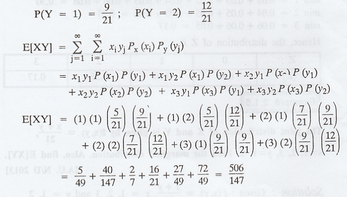
Example 2.1.5

The joint distribution of X and Y is given by f(x,y) = x+y/21, x = 1,2,3 y = 1,2. Find the marginal distribution. Also find E[XY] [A.U. N/D 2013]

Solution :

The marginal distribution of X :

The marginal distribution of Y :

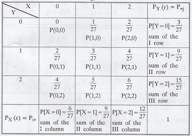
Example 2.1.6

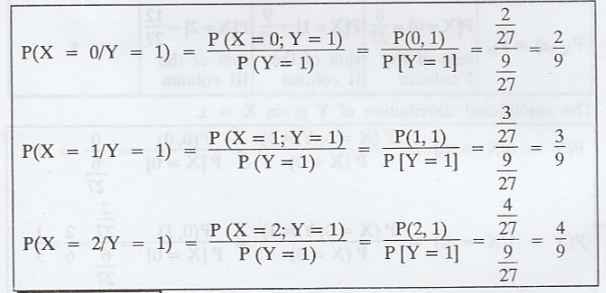
The two dimensional random variable (X, Y) has the joint density function f(x, y) = x +2y/27, x = 0, 1, 2 ; y = 0, 1, 2. Find the conditional distribution of Y given X = x. Also, find the conditional distribution of X given Y = 1. [A.U Tvli. A/M 2009] [A.U N/D 2017 R13-RP]

Solution:

Given: f(x, y) = x + 2y/27, x = 0, 1, 2 ; y = 0, 1, 2

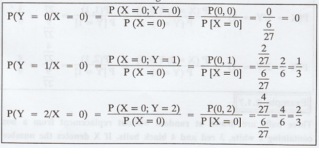
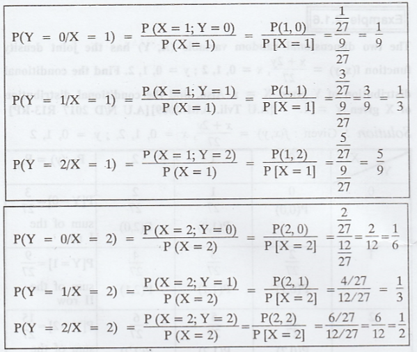
The conditional distribution of Y given X = x

The conditional distribution of X given Y = 1

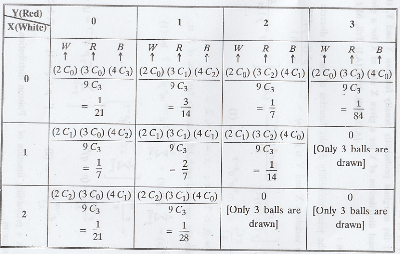
Example 2.1.7

Three balls are drawn at random without replacement from a box / containing 2 white, 3 red and 4 black balls. If X denotes the number of white balls drawn and Y denote the number of red balls drawn, find the joint probability distribution of (X, Y). [AU M/J 2007] [A.U A/M 2015 (RP) R-8] [A.U M/J 2016 RP R13]

Solution:

Three balls are drawn out of 9 balls.

X -> number of white balls drawn.

Y -> number of red balls drawn.

Example 2.1.8

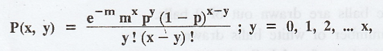
Two discrete r.v.'s X and Y have the joint probability density function; 

 x = 0, 1, 2, where m, p are constants with m > 0 and 0 < p < 1. Find (i) the marginal probability density function X and Y, (ii) the conditional distribution of Y for a given X and of X for a given Y. [A.U. N/D. 2005] [A.U Tvli. M/J 2010]

Solution :

Given the joint probability density function of the two discrete random variables X and Y is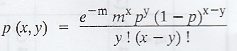 

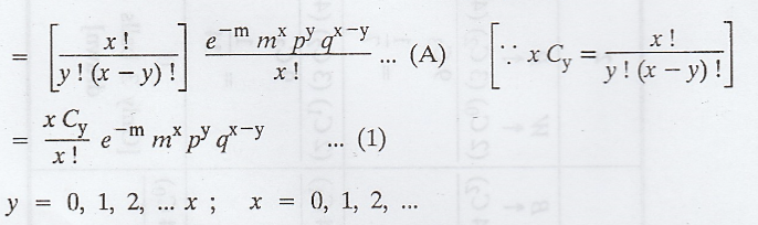
(i) Then the marginal probability density function of X is,

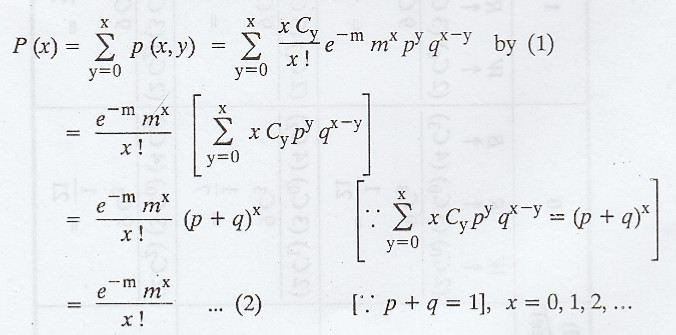
which is a probability function of a Poisson distribution with parameter m.

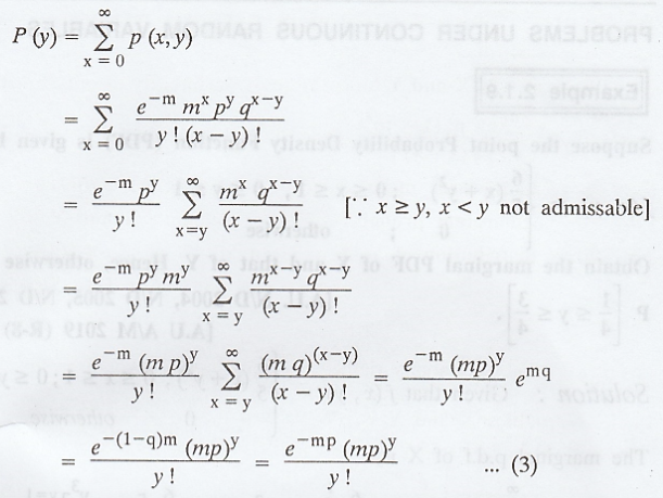
which is the probability function of a Poisson distribution with parameter (mp).

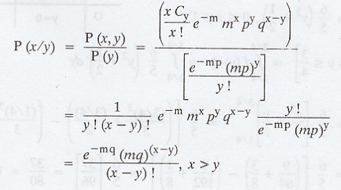
(ii) The conditional distribution of Y for given X is,

And the conditional probability distribution of X given Y is,