Introduction of Linear Time Invariant - Continuous Time Systems

LINEAR TIME INVARINT-CONTINUOUS TIME SYSTEMS

INTRODUCTION

A system is defined as an entity that acts on input signal and transforms it into an output signal. The most two attributes of a system are linearity and time invariance. A system which is both linear and time invariant is caused a linear time invariant (LTI) system.

Linear time invariant continuous time systems (LTI-CT) are characterized by

1) Differential equation

2) Block diagram                                                    

3) Impose response

4) Transfer function

5) State variable description

DIFFERENTIAL EQUATION

The general form of a constant co efficient differential equation is

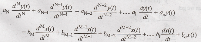
Here N is the order of the differential equation. x(t) is the input and y(t) is the output

(i) Zero state response

(ii) Zero input response.

The zero-state response of the system is the response due to the input when the initial state of the system is zero, on the other hand the zero-input response of the system is the response due to initial state of the system. In the second method, the output of an LIT continuous time system can be obtained using convolution integral.

Solution of differential equation

The general form of a Nth order differential equation is given by,

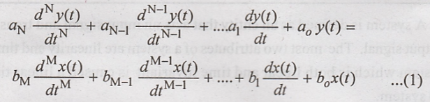
Where a_i and b_i are real constants and a_N ≠ 0

All practical system have M ≤ N

Total response = zero input response + zero state response.

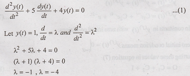
Natural response

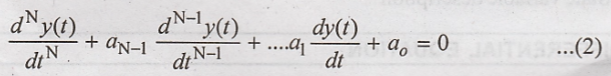
The natural response is the solution of equation (1) with x(t) = 0. This solution is also known as homogenous solution and is denoted by y⁽ⁿ⁾(t), equating the input terms in equation (1)

Let us assume the solution of equation (2) is of the form*

Substituting these result in equation (2) yields.

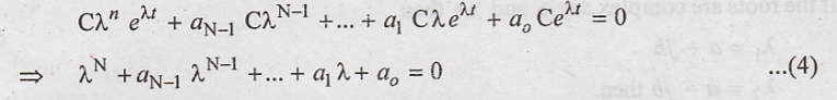
This polynomial is called the characteristic equation of the system

This equation (4) can be represented in factorized form as

Where λ₁, λ₂ are the roots of the characteristic equation roots, or eigen values or poles of the system. The nature of the response depends on the type of these roots.

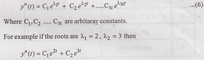
Distinct roots

If the roots λ₁, λ₂ ..., λ_N of equation (5) are distinct then the solution has the terms 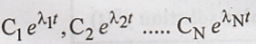. Therefore the solution is the form.

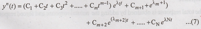
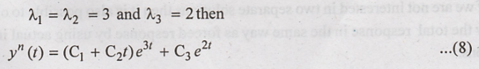
Repeated roots

If a root λ₁ is repeated m times (root of Multispecialty m) and remaining (N-M) roots are distinct then, the general solution is of the form

For example if the roots of characteristic equations are

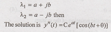
Complex roots

If the roots are complex say λ and λ* then

Forced response

The forced response of an LIT continuous time system is the response of the system when the initial conditions are zero. The forced response of the system is also known as zero-state response. It consists of, homogenous solution and particular solution. The form of homogeneous solution can be obtained from the roots of characteristic equation. The particular solution y(t) should satisfy the differential equation. The particular solutions for different types of inputs are given in the below table.

The forced response of the system is obtained by adding particular solution and homogeneous solution and then finding the coefficients of the homogeneous solution so that the combined response yⁿ(t) + y^p(t) satisfies the zero initial conditions.

Total response

The total response is obtained by adding the natural response and forced response that is

y(t) = yⁿ(t) + y^f(t)

If we are not interested in two separate solutions then it is also possible to obtain directly the total response in the same way as forced response by using actual initial conditions.

Problem 1:

An LTI CT system is specified by the following equation, 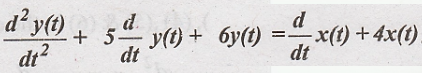. Find the following (i) The input x(t) is e^-t u(t) find the natural response for the initial condition 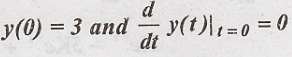 (ii) Forced response (iii) Total response.

Solution:

To find natural response:

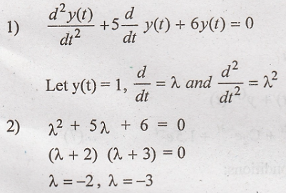
3) Homogeneous solution:

Apply initial conditions, y(0) = 3

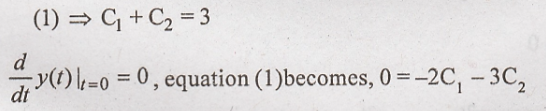
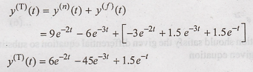
From the above equation we get C₁ = 9, C₂= 6, substitute in (1)

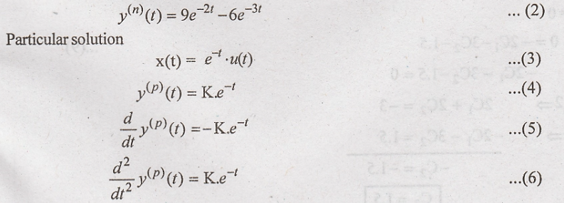
The particular solution should satisfy the given differential solution, so substitute (3), (4), (5) & (6) in the equation (1)

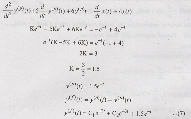
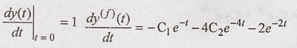
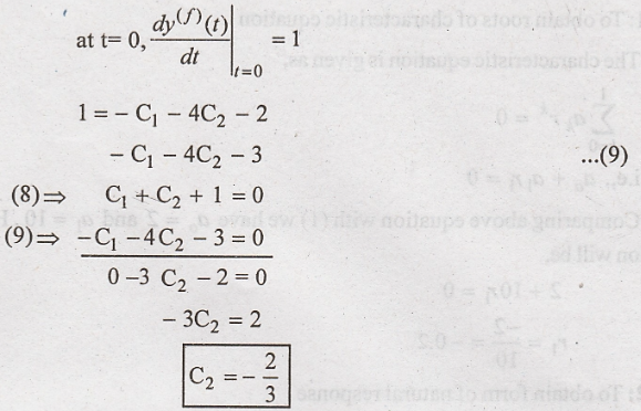
To obtain constants in y^(f)(t) with zero initial conditions:

Zero initial condition means  putting these value in equation (7)

Differentiate equation (7) with respect to 't'.

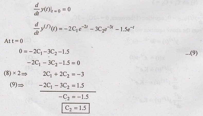
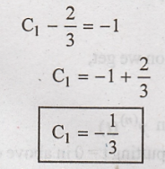
Substitute C₂ in equation (8)

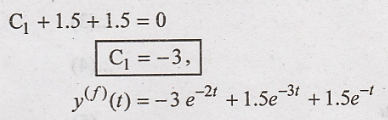
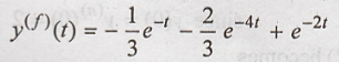
Total response:

Problem 2:

An LTI system is represented by 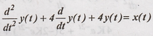 with initial conditions 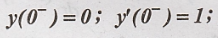find the output of the system, when the input is x(t) = e^t a(t).

Solution:

The given different equation is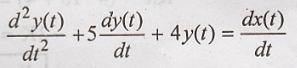 

The complete response will be given as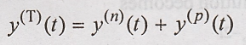 

To find natural response,

Homogeneous solution:

To find particular solution

The particular solution should satisfy the given differential equation so substitute (3), (4), (5) & (6) in the given equation

Hence the particular solution becomes

To obtain constants in y^(f)(t) with zero initial conditions:

Differentiate equation (7) with respect to 't' O = C₁ + C₂ + 1

Substitute C₂ in equation (8)

Substitute the values of C₁ and C₂ in equation (7)

This is the complete response of the given system.

Problem 3:

Determine the natural response of the system described by differential equation 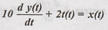with y(0) = 2.

Solution:

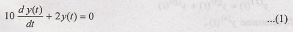
The natural response is obtained with zero input. Hence the homogeneous differential equation becomes,

Step 1: To obtain roots of characteristic equation

The characteristic equation is given as,

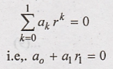
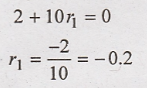
Comparing above equation with (1) we have a₀ = 2 and a₁ = 10. Hence above equation will be,

Step 2: To obtain form of natural response

Since the root of characteristic equation is real,

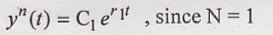
Putting the value of r₁ in above equation we get,

Step 3: To obtain values of constants in y⁽ⁿ⁾(t)

The initial condition is y(0) = 2, putting t = 0 in above equation,

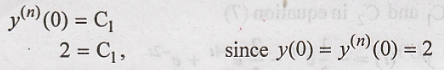
Hence the equation (2) becomes

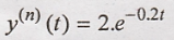
This is the natural response of the given system.

Problem 4:

Determine the forced response of the system 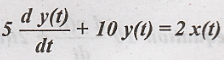 for the input x(t) = 2 u(t).

Solution:

The forced response of the system is obtained only with inputs. It is given as

Step 1: To obtain roots of characteristic equation

For the order N = 1,

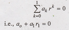
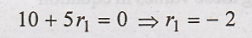
Comparing above equation with equation (1), we have a₀ = 10 and a₁ = 5r₁ Hence above equation will be,

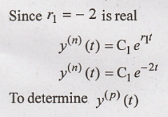
Step 2: To obtain form of natural response

Step 3: Form of particular solution

The particular solution is of the same form of input. Here x(t) = 2 u(t), i.e. Constant. Hence the particular solution will be of the form,

y^(p)(t) = k

Step 4: To obtain values of constants in y^(p)(t)

Now we have to determine the value of k for which y^(p)(t) satisfies the systems differential equation. Hence putting

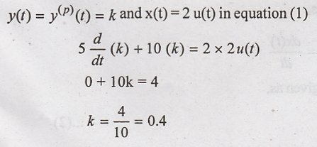
Hence the particular solution becomes,

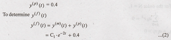
Step 5: Obtain constants in y^(f)(t) with zero initial conditions

Zero initial conditions means y^(f)(0) = 0. Putting these values in equation

0 = C₁ + 0.4

C₁ = -0.4

Hence equation (2) becomes,

This is the forced response of the given system

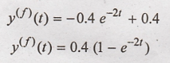
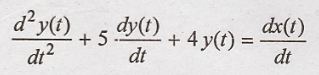
Problem 5:

Determine the complete response of the system:

Solution:

The given differential equation is,

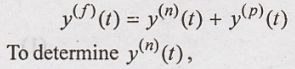
The complete response will be given as,

To determine y⁽ⁿ⁾(t)

Step 1: Roots of characteristic equation

Here N = 2, hence from given differential equation we can write,

r² + 5r + 4 = 0

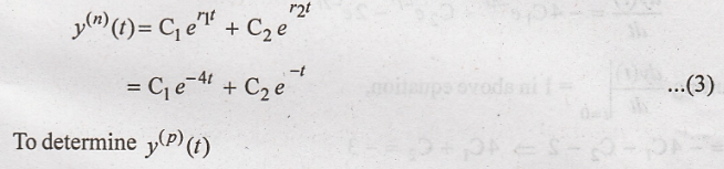
Roots of this equation will be,

r₁ = - 4 and r₂ = -1

Step 2: Form of natural response

For real roots.

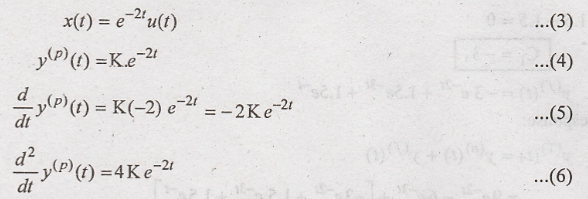
Step 3: Form of particular solution

The input is x(t) = e^-2t u(t). Hence the particular solution will be of form,

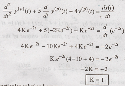
Step 4: Values of k

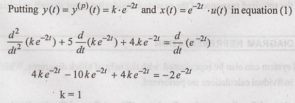
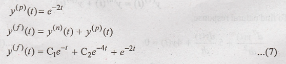
Hence particular solution becomes (putting k = 1 in equation (4)

To determine y(t)

Putting y^(p)(t) from above equation and y⁽ⁿ⁾(t) from equation (3) in equation (2)

We get natural response as,

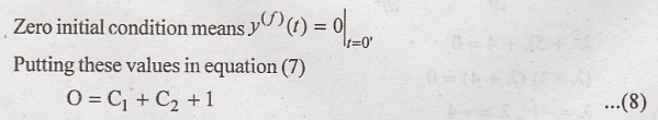
Step 5:

Values of C₁ and C₂ with initial conditions

Putting y(0) = 0 above equation

0 = C₁ + C₂ + 1 ⇒ C₂ = -1

Differentiate equation (6) with respect to 't',

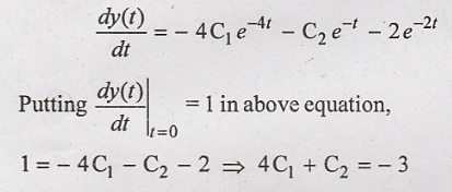
Solving above equation and equation (7) for C₁ and C₂ we get,

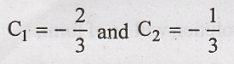
Here the complete response becomes (by putting C₁ and C₂ in equation (6)

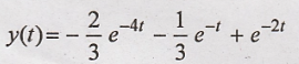
This is the required response of the system considering input as well as initial conditions.