Introduction of Analysis of Discrete Time Signals

INTRODUCTION OF ANALYSIS OF DISCRETE TIME SIGNALS

Most of the signals encountered in nature are continuous in time but in digital signal processing the signals are sampled and quantized at discrete-time instants and are represented as a sequence of 1's and O's. For example, signal such as speed signal, ECG and EEG are electrical signals and therefore necessary to perform a conversion to digital representation. This can be done by an analog to digital representation. This can be done by an analog to digital converter.

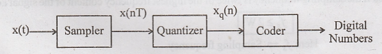
The above figure shows the ADC unit and its constituent parts. The sampler, samples the input signal with a sampling interval T, producing an output x(nT). The signal x(nT) is discrete in time but continuous in amplitude. The output of the sampler is applied to a quantize. It converts x(nT) into discrete time, discrete-amplitude signal. After sampling and quantization, the final step in converting an analog signal to a form acceptable to digital computer is called coding. The coder maps each quantized sample value in digital world.

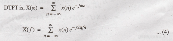
A continuous time signal can be represented in the frequency domain using Laplace transform or continuous-time Fourier transform (CTFT). Similarly, a discrete time signal can be represented in the Frequency domain using Z- transform or discrete time Fourier transform. The Fourier transform of a discrete time signal is called discrete time Fourier transform (DTFT).

BASEBAND SAMPLING

Sampling Theorem for Lowpass (LP) Signals

Statement of sampling Theorem:

1. A band limited signal of finite energy, which has no frequency components higher than W hertz, is completely described by specifying the values of the signal at instants of time separated by 1/2W seconds.

2. A bandlimited signal of finite energy, which has no frequency components higher than W hertz, may be completely recovered from the knowledge of its samples taken at the rate of 2W samples per second.

The first part of above statement tells about sampling of the signal and second part tells about reconstruction of the signal. Above statement can be combined and stated alternatively as follows:

A continuous time signal can be completely represented in its samples and recoved back if the sampling frequency is twice of the highest frequency content of the signal i.e.,

f_s ≥ 2W

Here f_s ⇒ Sampling frequency

W ⇒ Higher frequency content

Proof of Sampling theorem:

There are two parts:

(i) Representation of x(t) intems of its samples.

(ii) Reconstruction of x(t) from its samples.

Part I: Representations of x(t) intems of its samples. x(n T_s)

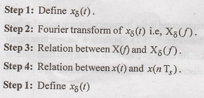
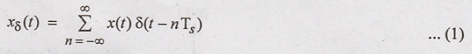
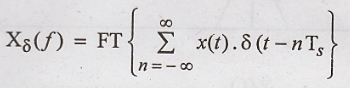
The sampled singal x_δ (t) is given as

Step 2: 

Taking FT of equation

We know that FT of product in time domain becomes convolution in frequency domain. i.e.,

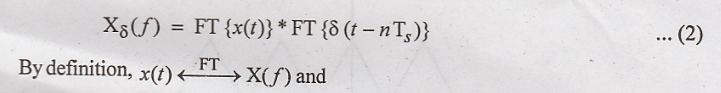
Hence equation (2) becomes,

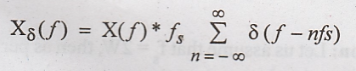
Since convolution is linear

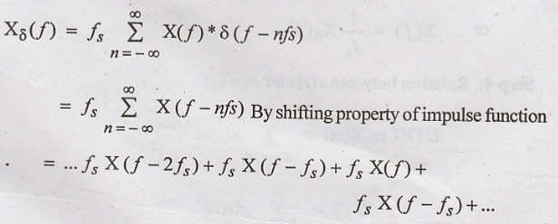
Comments:

(i) The RHS of above equation shows that X(f) is placed at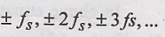 

(ii) This means X(f) is periodic in f_s.

(iii) If sampling frequency is f_s = 2W, then the spectrum X(f) just touch each other.

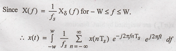
Step 3: Relation between X(f) and X_δ(f).

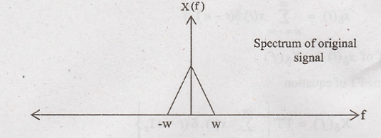
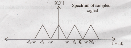
Important assumption: Let us assume that fs = 2W, then as per above diagram,

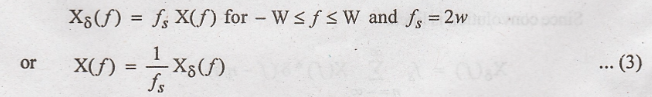
Step 4: Relation between x(t) and x(nT_s).

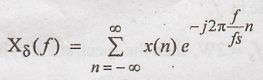
In above equation f is the frequency of DT signal. If we replace X(f) by X_δ(f), then 'f becomes frequency of CT signal i.e.,

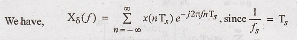
In above equation f is frequency of CT signal and f/f_s = frequency of DT signal in equation since x(n) = x(nT_s), i.e. samples of x(t), then

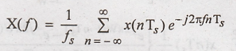
Putting above expression in equation (3)

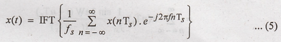
Inverse Fourier transform (IFT) of above equation gives x(t) i.e.,

Comments:

i) Here x(t) is represented completely interms of x(nT_s).

ii) Above equation holds for f_s = 2W. This means if the samples are taken at the rate of 2W or higher, x(t) is completely represented by its samples.

iii) First part of the sampling theorem is proved by above two comments.

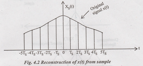
Part-II: Reconstruction of x(t) from its samples.

Step 1: Take inverse Fourier transform of X(f) which is interms of X_δ(f).

Step 2: Show that x(t) is obtained back with the help of interpolation function.

Step 1: The IFT of equation (5) becomes,

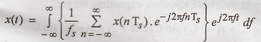
Here the integration can be taken from - W ≤ f ≤ W.

Interchanging the order of summation and integration,

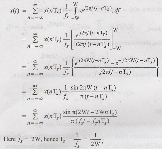
Simplifying above equation,

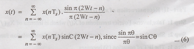
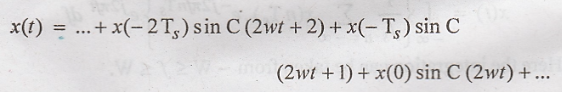
Step 2: Let as interpret the above equation, expanding we get,

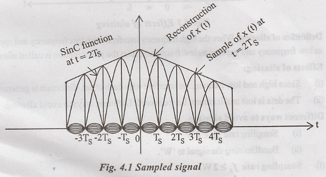
Comments:

(i) The samples x(nT_s) are weighted by SinC function.

(ii) The SinC function is the interpolating function

Step 3: Reconstruction of x(t) by low pass filter

Effects of Undersampling (Aliasing)

While proving sampling theorem we considered that f_s = 2W consider the case of f_s < 2 W, then spectrum of X_δ(f) will be modified as follows:

(i) The spectrum located at X(ƒ), X(f − ƒ_s), X(ƒ −2ƒ_s), ... overlap on each other.

(ii) Consider the spectrums of X(f) and X(f - f_s) is magnified.

(iii) The high frequencies near 'ω' in X(f - f_s) overlap with low frequencies (f_s - W) in X(f).

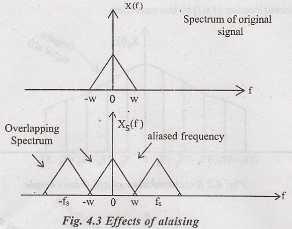
Definition of aliasing: When the high frequency interferes with low frequency and appears as low frequency and appears as low frequency, then the phenomenon is called aliasing.

Effects of aliasing:

(i) Since high and low frequencies interfere with each other, distortion is generated.

(ii) The data is lost and it cannot be recovered. Different ways to avoid aliasing.

Different ways to avoid aliasing

(i) Sampling rate f_s ≥ 2W

(ii) Bandlimitting the signal to 'W'.

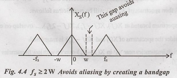
(i) Sampling rate f_s ≥ 2W

When the sampling rate is made higher than 2W, then the spectrums will not overlap and there will be sufficient gap between the individual spectrum.

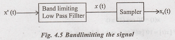
(ii) Bandlimitting the signal

The sampling rate is, f_s = 2 W. There can be for components higher than 2W. These components creating aliasing. Hence a low pass filter is used before sampling the signal as shown in figure.

Nyquist rate and Nyquist interval

Nyquist rate: When the sampling becomes exactly equal to '2W' samples/sec, for a given bandwidth of W hertz, then it is called Nyquist rate.

Nyquist interval: It is the time interval between any two adjacent samples when sampling rate is Nyquist rate.

Nyquist rate = 2W Hz

Nyquist interval = 1/2W seconds

Problem based on sampling theorem

Problem 1:

A signal having a spectrum ranging from near dc to 10KHz is to be sampled and converted to discrete form. What is the minimum number of samples per second that must be taken to ensure recovery?

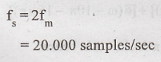
Solution:

Given: f_m = 10 KHz

From Nyqulist rate, the minimum number of samples that must be taken to ensure recovery is,

Problem 2:

The signal x(t) = 10 cos (10πt) is sampled at a rate 8 samples per second. Plot the amplitude spectrum for w≤ 30 π. Can the original signal can be recovered from samples? Explain.

Solution:

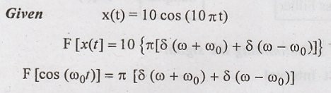
The amplitude spectrum shown below

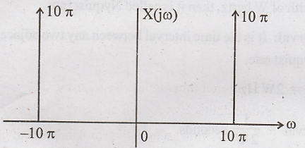
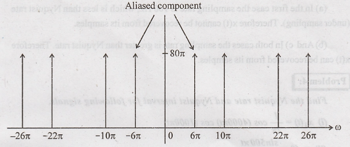
The sampling rate is less than Nyquist rate. So, the original signal cannot be recovered from the samples.

The frequency spectra of sampled x(t) is given by

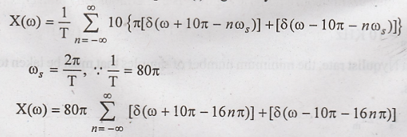
The plot of amplitude spectrum for |ω|≤ 30 π is shown in below

Problem 3:

A signal x(t) = sin C (150 πt) is sampled at a range of (a) 100 Hz (b) 200 Hz (c) 300 Hz. For each of these three cases, explain if you can recover the signal x(t) from the sampled signal.

Solution:

Given: x(t) = sinС (150 πt)

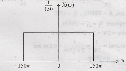
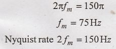
The spectrum of the signal x(t) is a rectangular pulse with a bandwidth (maximum frequency component) of 150 π rad/sec.

From the above figure, we have

(a) In the first case the sampling rate is 100 Hz, which is less than Nyquist rate (under sampling). Therefore x(t) cannot be recovered from its samples.

(b) And c) In both cases the sampling rate is greater than Nyquist rate. Therefore x(t) can be recovered from its samples.

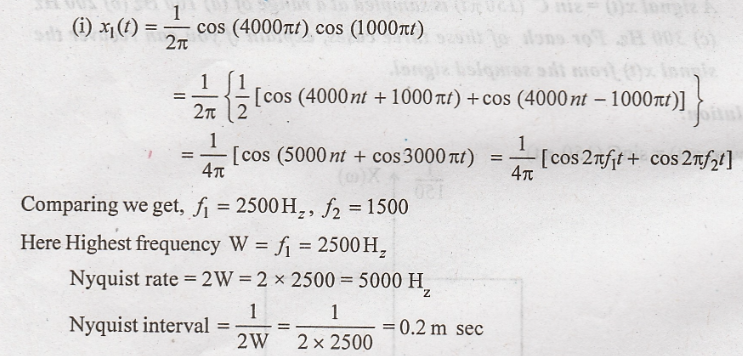
Problem 4:

Find the Nyquist rate and Nyquist interval for following signals.

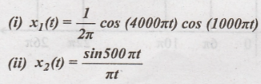
Solution:

Problem 5:

Determine the Nyquist sampling rate and Nyquist sampling interval for following signals:

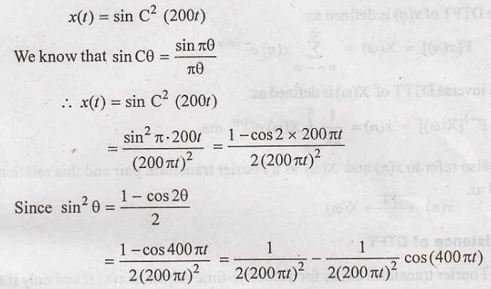
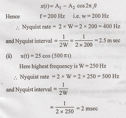
(i) x(t) = sin C² (200t)

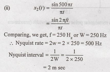
(ii) x(t) = 25 cos (500 πt)

Solution:

compare above equation with,