Covariance Correlation and Regression

COVARIANCE, CORRELATION AND REGRESSION

When two or more random variables are defined on a probability space, it is useful to describe how they vary together, that is, it is useful to measure the relationship between the variables. A common measure of the relationship between two random variables is the covariance. To define the covariance, we need to describe the expected value of a function of two random variables h (x, y). The definition simply extends that used for a function of a single random variable.

i. COVARIANCE

If X and Y are random variables, then co-variance between them is defined as, [A.U N/D 2019 (R17) PS]

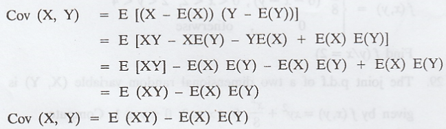
Note: If X and Y are independent, then Cov (X, Y) = 0

If X and Y are independent, then E [XY] = E(X). E(Y) => Cov (X, Y) = 0

ii. CORRELATION ANALYSIS

A distribution involving two variables is known as a bivariate distribution. If these two variables vary such that change in one variable affects the change in the other variable, the variables are said to be correlated. For example, there exists some relationship between the height and weight of a person, price of a commodity and its demand, rainfall and production of rice, etc. The degree of relationship between the variables under consideration is measured through the correlation analysis. The measure of correlation is called as the correlation co-efficient or correlation index. Thus, the correlation analysis refers to the techniques used in measuring the closeness of relationship between the variables.

Types of correlation

There are three important ways of classifying correlation viz.,

a. Positive and Negative

b. Simple, partial and multiple

c. Linear and non-linear.

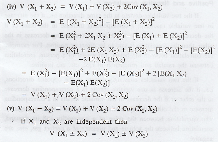
a. Positive and Negative correlation :

If the two variables deviate in the same direction i.e., if the increase in one variable results in a corresponding increase in the other or if the decrease in one variable result in a corresponding decrease in the other, then the correlation is said to be direct or positive. For example, the correlation between the height and weight of a person, correlation between the rainfall and production of rice, etc. are positive.

If the two variables constantly deviate in the opposite directions, i.e., if the increase in one variable results in a corresponding decrease in the other or if the decrease in one variable results in a corresponding increase in the other, the correlation is said to be inverse or negative. The correlation between the price of a commodity and its demand, correlation between the volume and pressure of a perfect gas, etc., are negative.

Correlation is said to be perfect if the deviation in one variable is followed by a corresponding and proportional deviation in the other.

b. Simple, partial and multiple correlation :

If only two variables are considered for correlation analysis, it is called a simple correlation. When three or more variables are studied, it is a problem of either multiple or partial correlation.

In multiple correlation, three or more variables are studied simultaneously. For example, the study of relationship between the yield of rice per hectare and both the amount of rainfall and the usage of fertilizers is a multiple correlation.

When three or more variables are involved in correlation analysis, the correlation between the dependent variable and only one particular independent variable is called partial correlation. The influence of other independent variable is excluded.

For example, the yield of rice is related with the application of fertilizers and the rainfall. In this case, the relation of yield to fertilizer excluding the effect of rainfall, the relation of yield to rainfall excluding the usage of fertilizer are partial correlations.

c. Linear and non-linear correlation :

If the amount of change in one variable tends to bear constant ratio to the amount of change in the other variable, then the correlation is said to be linear.

For example, if

the variation between X and Y is a straight line

A correlation is said to be non-linear or curvi linear if the amount of change in one variable does not bare a constant ratio to the amount of change in the other variable. For example, if rainfall is doubled, the production of rice would not necessarily be doubled.

Methods of studying correlation :

as The following are some of the methods used for studying the correlation.

(i) Scatter diagram method

(ii) Graphic method

(iii) Karl pearson's co-efficient of correlation

(iv) Rank method

(vi) Method of least squares.

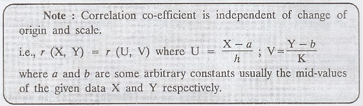
Karl Pearson's co-efficient of correlation :

Let X and Y be given random variables. The Karl Pearson's co-efficient of correlation is denoted by r_XY or r(X, Y) and defined as

Note that correlation co-efficient always lies between -1 to +1.

Note: Two random variables with non zero correlation are said to be correlated.

iii. RANK CORRELATION

Let us suppose that a group of 'n' individuals is arranged in order of merit or proficiency in possession of two characteristics A and B. These ranks in the two characteristics will, in general, be different. For example, if we consider the relation between intelligence and beauty, it is not necessary that a beautiful individual is intelligent also.

If (X_i, Y_i), i = 1, 2, ... n are the ranks of the individuals in two characteristics A and B respectively, then the rank correlation co-efficient is given by,

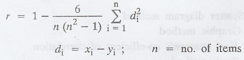
where d_i is the different between the ranks. This formula is called Karl Pearson's formula for the rank correlation co-efficient.

iv. REPEATED RANKS

If any two or more individuals are equal in any classification with respect to characteristic A or B, or if there is more than one item with the same value in the series then Spearman's formula for calculating the rank correlation coefficients breaks down. In this case common ranks are given to the repeated ranks. This common rank is the average of the ranks which these items would have assumed if they are slightly different from each other and the next item will get the rank next to the ranks already assumed. As a result of this, following adjustment or correction is made in the correlation formula.

In the correlation formula, we add the factor 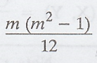 ∑d² where m is the number of times an item is repeated. This correction factor is to be added for each repeated value.

Example 2.2.1

Calculate the correlation co-efficient for the following heights (in inches) of fathers X and their sons Y. [A.U. N/D 2004, A/M 2015 (RP) R13]

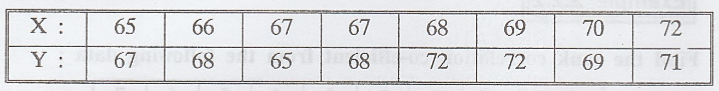
Solution :

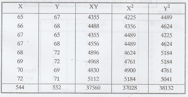
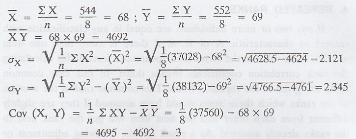
The correlation co-efficient of X and Y is given by,

Example 2.2.2

Find the rank correlation co-efficient from the following data:

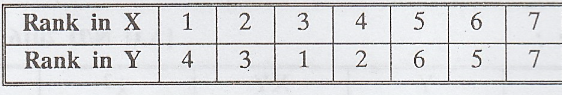
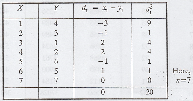
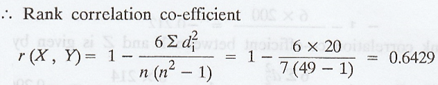
Solution :

Example 2.2.3

Ten participants were ranked according to their performance in a mustical test by the 3 Judges in the following data.

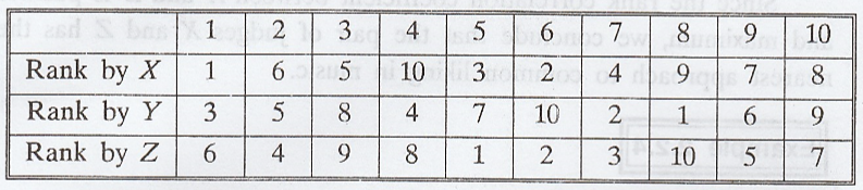
Using rank correlation method, discuss which pair of judges has the nearest approach to common likings of music.

Solution :

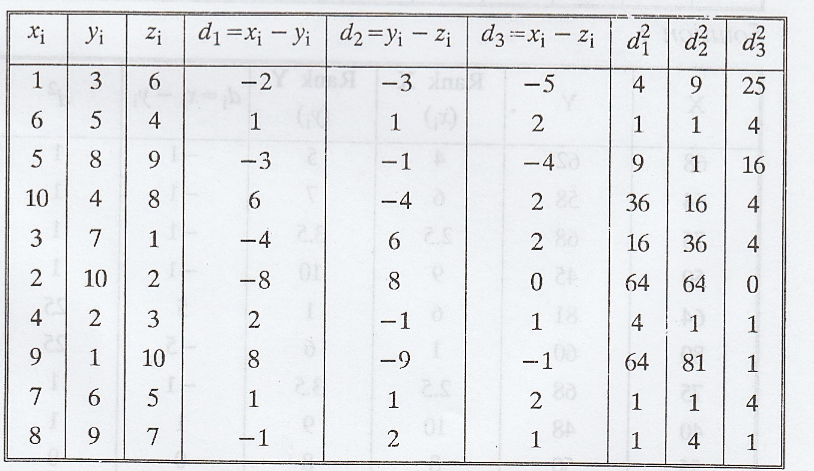
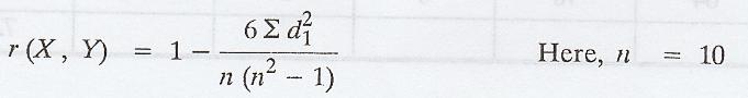
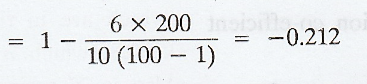
The rank correlation co-efficient between X and Y is given by

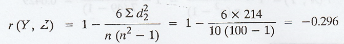
The rank correlation co-efficient between Y and Z is given by

The rank correlation co-efficient between X and Z is given by

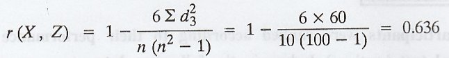
Since the rank correlation coefficient between X and Z is positive and maximum, we conclude that the pair of judges X and Z has the nearest approach to common liking in music.

Example 2.2.4

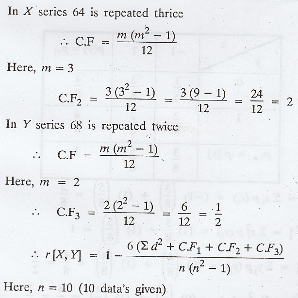
Obtain the rank correlation coefficient for the following data:

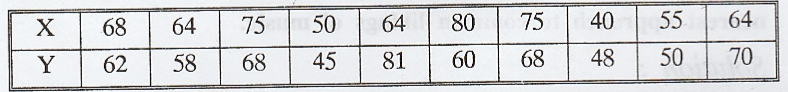
Solution :

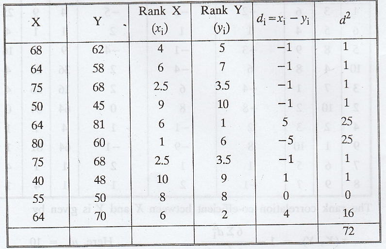
In X series 75 is repeated twice which are in the positions 2^nd and 3^rd ranks. Therefore common ranks 2.5 (which is the average of 2 and 3) is to be given for each 75. Also in X series 64 is repeated thrice which are in the position 5^th, 6^th and 7^th ranks.

Therefore common ranks 6 (which is the average of 5, 6 and 7) is to be given for each 64.

Similarly in Y series 68 is repeated twice which are in the positions 3^rd and 4^th ranks. Therefore common ranks 3.5 (which is the average of 3 and 4) is to be given for each 68.

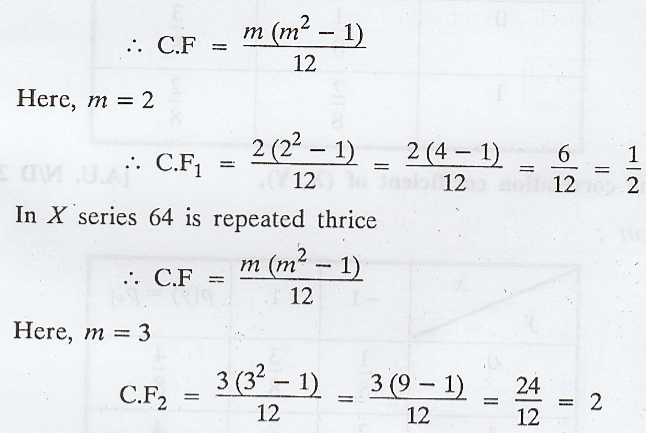
Correction factors

In X series 75 is repeated twice

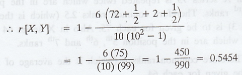
Example 2.2.5

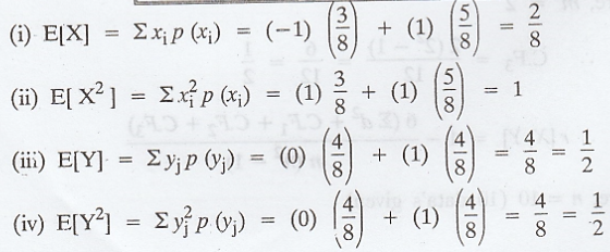
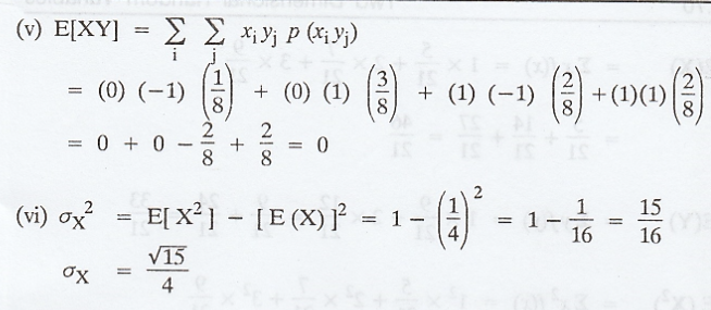
The joint probability mass function of X and Y is given below.

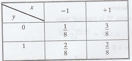
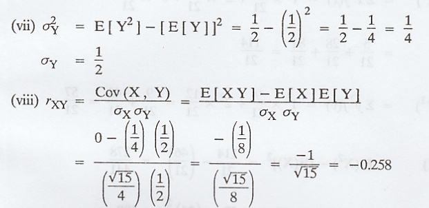
Find the correlation coefficient of (X, Y).

Solution :

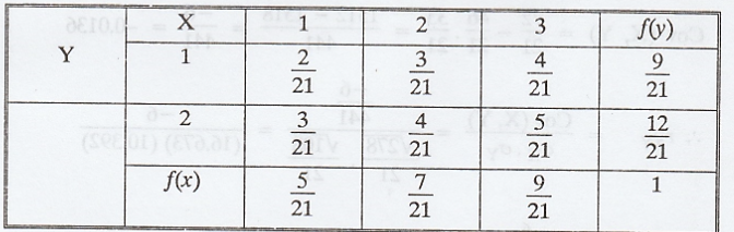
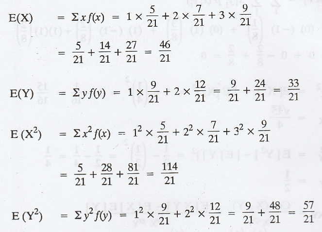
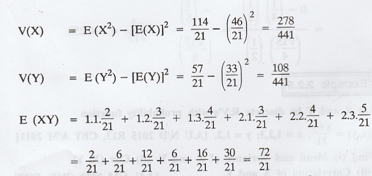
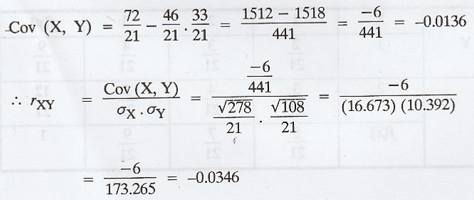
Example 2.2.6

Let X and Y be discrete R.V's with probability function f(x,y) = x+y/21, x=1,2,3; y=1,2. Find (i) Mean and Variance of X and Y. (ii) Cov (X, Y) (iii) Correlation of X and Y. [A.U N/D 2015 R13, CBT A/M 2011], [A.U A/M 2019 (R17) PQT]

Solution :

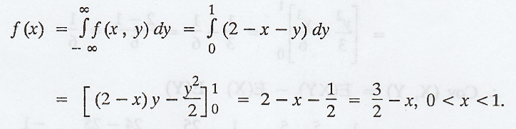
Example 2.2.7

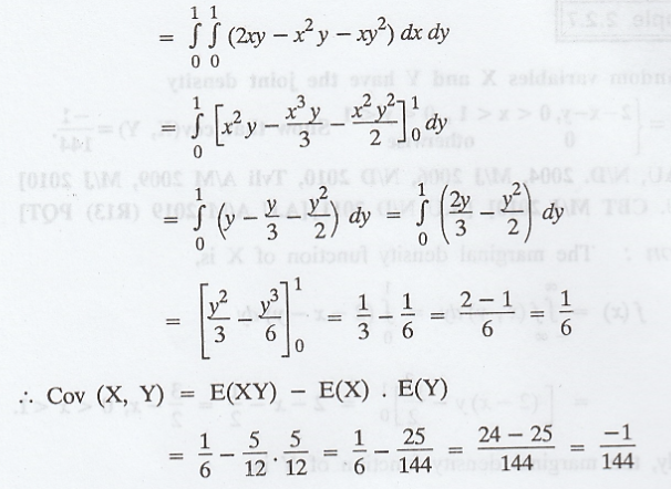
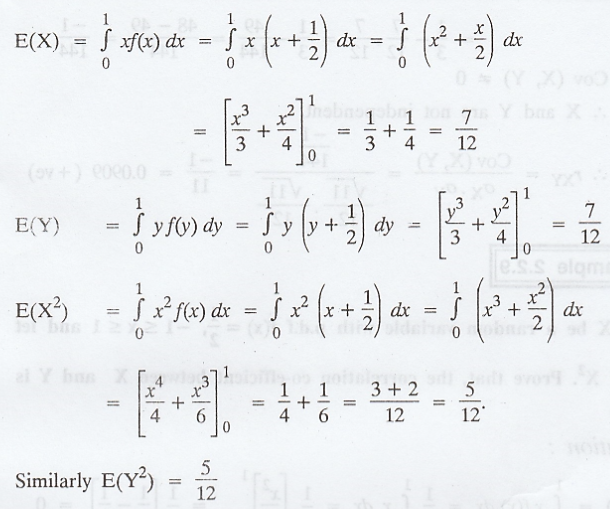
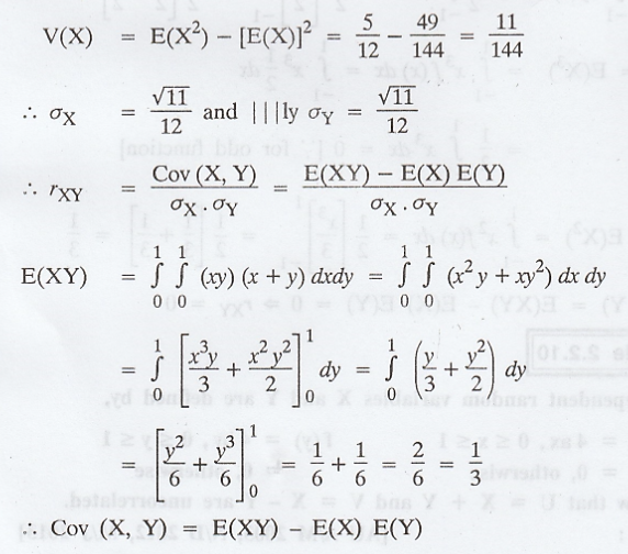
Two random variables X and Y have the joint density 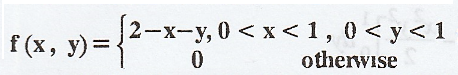 Show that cov(X, Y) = -1/144. [AU, N/D. 2004, M/J 2006, N/D 2010, Tvli A/M 2009, M/J 2010] [A.U. CBT M/J 2010] [A.U N/D 2011] [A.U A/M 2019 (R13) PQTI

Solution :

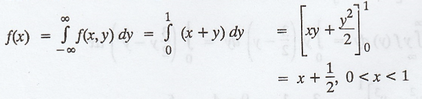
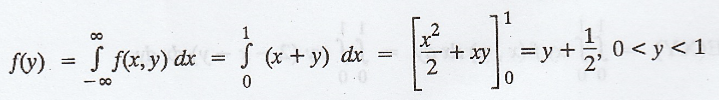
The marginal density function of X is,

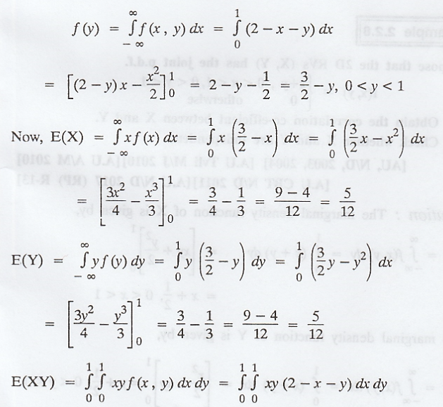
Similarly, the marginal density function of Y is,

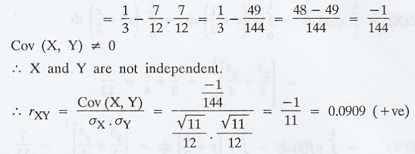
Example 2.2.8

Suppose that the 2D RVs (X, Y) has the joint p.d.f. 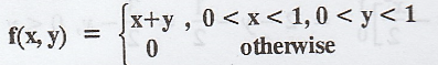 Obtain the correlation co-efficient between X and Y. Check whether X and Y are independent. [AU, N/D, 2003, 2004] [A.U Tvli M/J 2010] [A.U A/M 2010] [A.U CBT N/D 2011] [A.U N/D 2017 (RP) R-13]

Solution:

The marginal density function of X is given by,

The marginal density function of Y is given by,

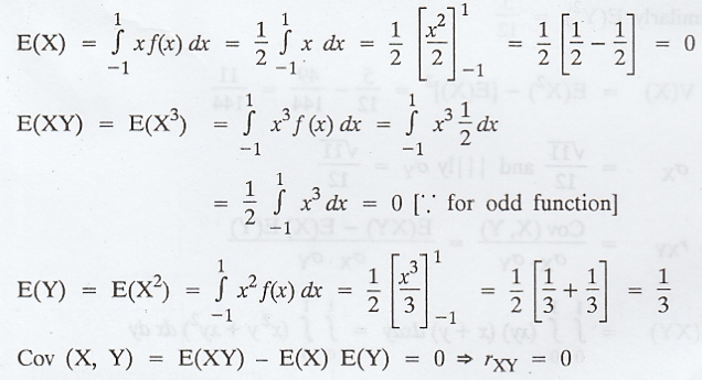
Example 2.2.9

Let X be a random variable with p.d.f f(x) = 1/2, -1 ≤ x ≤ 1 and let Y = X². Prove that, the correlation co-efficient between X and Y is zero.

Solution :

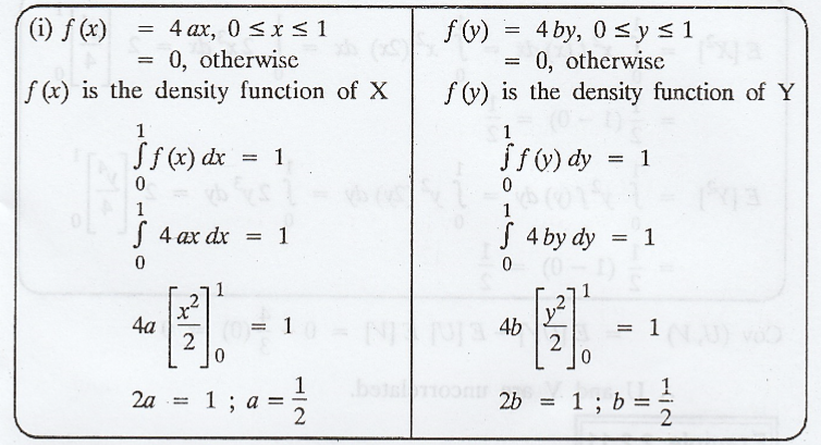
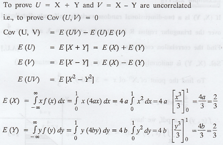
Example 2.2.10

Two independent random variables X and Y are defined by,

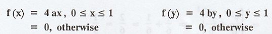
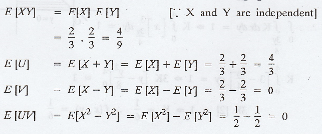
Show that U = X + Y and V = X - Y are uncorrelated. [AU A/M 2003, N/D 2012, M/J 2013]

Solution :

 

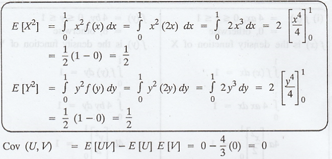
.'. U and V are uncorrelated.

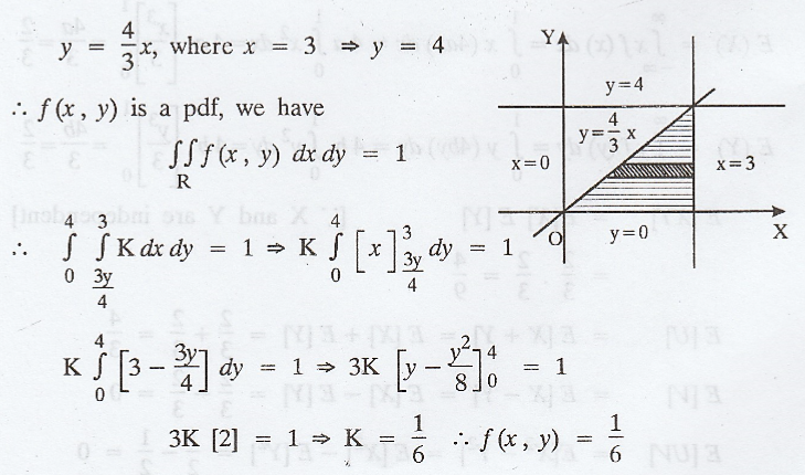
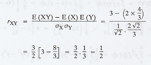
Example 2.2.11

If (X, Y) is a two-dimensional random variable uniformly distributed over the triangular region R bounded by y=0, x = 3, and y =4x/3. Find the correlation coefficient r_xy. [A.U.]

Solution:

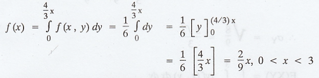
(X, Y) is uniformly distributed, f (x, y) = K, constant (say)

To find the point of Xⁿ of x = 3 and y = 4x/3

The marginal density function of X is

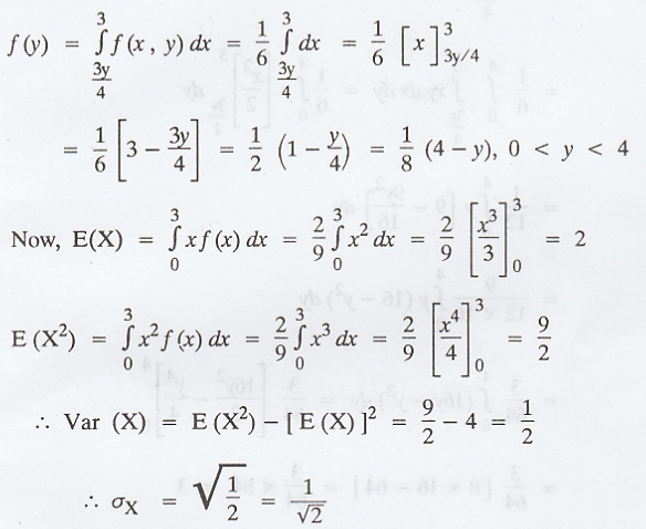
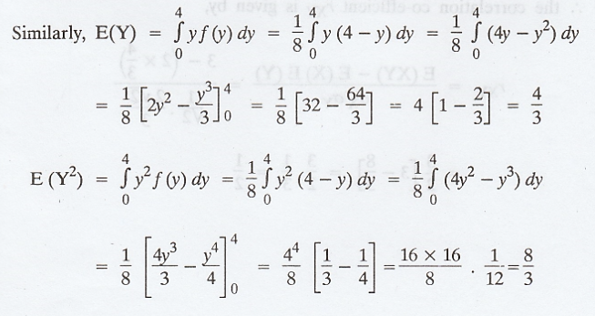
similarly the marginal density function of Y is

 

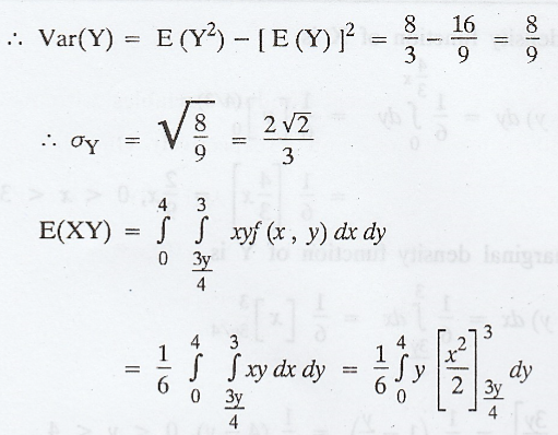
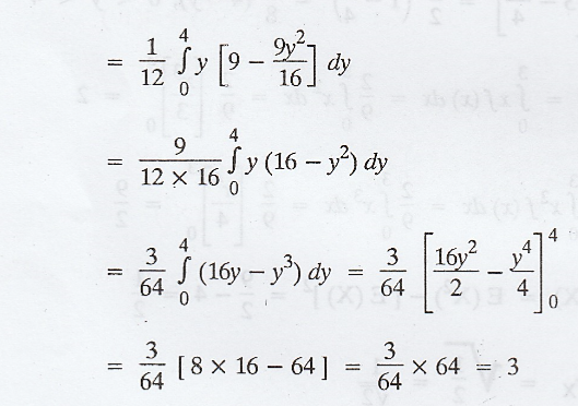
.'. the correlation co-efficient r_XY is given by,

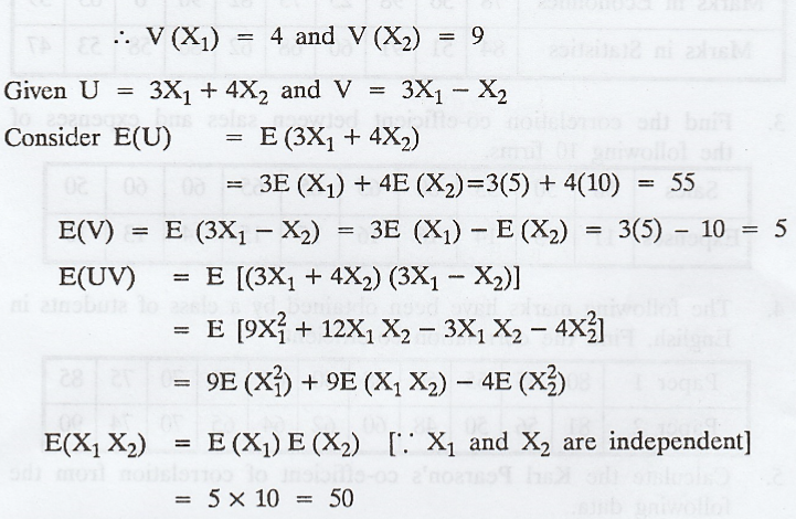
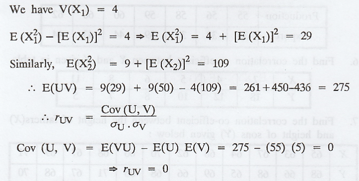
Example 2.2.12

Let X₁ and X₂ be two independent random variables with means 5 and 10 and standard deviations 2 and 3 respectively. Obtain r_UV where U = 3X₁ + 4X₂ and V = 3X₁ - X₂. [A.U N/D 2019 (R17) PS]

Solution:

EXERCISE 2.2

1. For the given data, find the correlation co-efficient between X and Y.

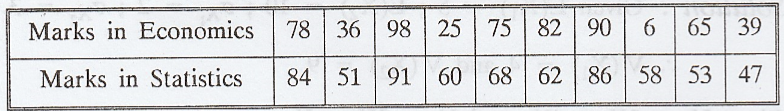
2. Ten students got the following percentage of marks in Economics and Statistics. Calculate the correlation co-efficient.

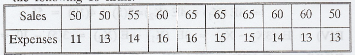
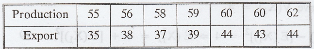
3. Find the correlation co-efficient between sales and expenses of the following 10 firms.

4. The following marks have been obtained by a class of students in English. Find the correlation co-efficient.

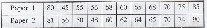
5. Calculate the Karl Pearson's co-efficient of correlation from the following data.

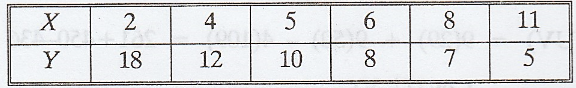
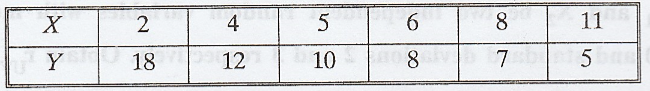
6. Find the correlation co-efficient between X and Y given in table.

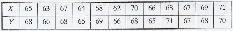
7. Find the correlation co-efficient between the height of fathers(X) and height of sons (Y) given below:

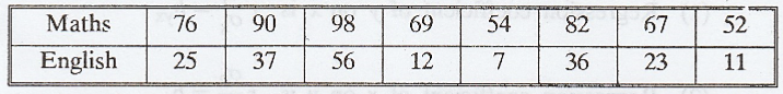
8. Find the rank correlation co-efficient of ranks of 8 candidates in Maths and English as given below :

9. Let the random variable X have the marginal density function g(x) = 1, -1/2 < x < 1//2 and let the conditional density of Y be

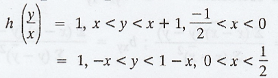 S.T the variables X and Y are uncorrelated.

10. Let X and Y be random variables having joint density function 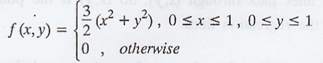 Find r_XY.

11. If ƒ (x, y) = 1/8 (6 - x - y), 0 ≤ x ≤ 2, 2 ≤ y ≤ 4, find r_XY.