Central Limit Theorem

CENTRAL LIMIT THEOREM

[for independent and identically distributed random variables]

The most widely used model for the distribution of a random variable is a normal distribution. Whenever a random experiment is replicated, the random variable that equals the average result over the replicates tends to have a normal distribution as the number of replicates becomes large. De Moivre presented this fundamental result, known as the central limit theorem, in 1733.

The central limit theorem says that the probability distribution function of the sum of a large number of random variables approaches a gaussian distribution. Although the theorem is known to apply to some cases of statistically dependent random variables, most applications, and the largest body of knowledge are directed towards statistically independent random variables.

It not only provides a simple method for computing approximate probabilities for sums of independent random variables, but it also helps explain the remarkable fact that the empricial frequencies of so many natural populations exhibit bell shaped (that is, normal) curves.

The first version of the central limit theorem was proved by De Moivre around 1733. This was subsequently extended by Laplace (the Newton of France) Laplace also discovered the more general form of the central limit theorem which is given. His proof, however, was not completely rigorous and, in fact, cannot easily be made rigorous. A truly rigorous proof of the central limit theorem was first presented by the Russian mathematician Liapounoff in the period 1901 - 1902.

The application of the central limit theorem to show that measurement errors are approximately normally distributed is regarded as an important contribution to science. Indeed, in the seventeenth and eighteenth centuries the central limit theorem was often called the "law of frequency of errors".

i. Central Limit Theorem: [Lindberg-Levy's form] [A.U A/M 2004, N/D 2010, A/M 2010, N/D 2011] [A.U M/J 2013, N/D 2013]

Statement :

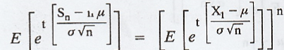
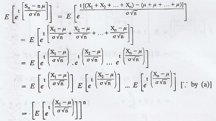
If X₁, X₂, ..., X_n be a sequence of independent identically distributed random variables with E [X_i] =µ and Var [X_i] = σ², i = 1, 2, ..., n and if S_n = X₁ + X₂ + ... + X_n, then under certain general conditions, S_n follows a normal distribution with mean 'nµ' and variance 'n σ²' as n → ∞

Proof

Given :

(a) X₁, X₂, X_n be 'n' independent and identically distributed r.v's

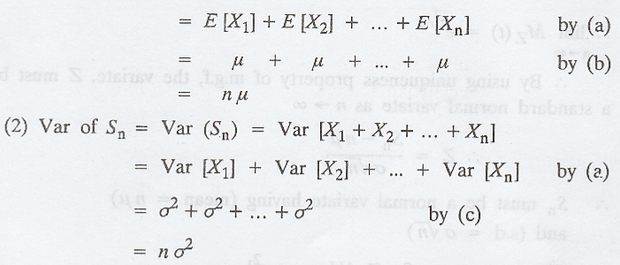
(b) E[X₁] = E [X₂] = E[X_n] = µ

(c) Var [X₁] = Var [X₂] = Var [X_n] = σ²

(d) S_n = X₁ + X₂ + ... + X_n

To prove :

(1) Mean of S_n = nµ

(2) Var [S_n] = n σ²

(3) S_n must be a normal variate with mean 'n µ' and s.d. ' σ √ n'

i.e. To prove :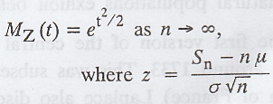 

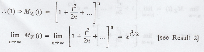
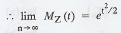
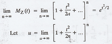
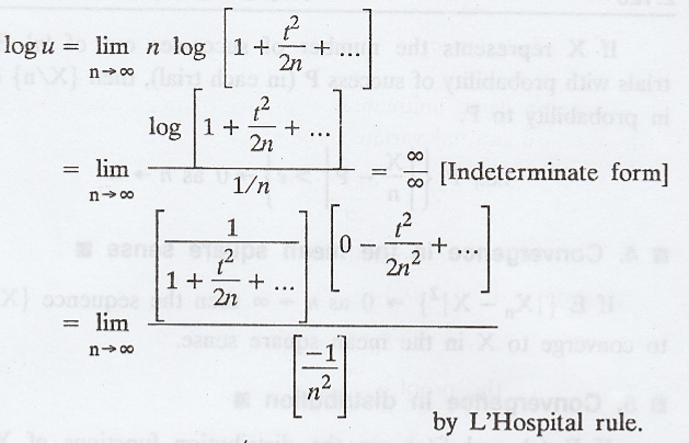
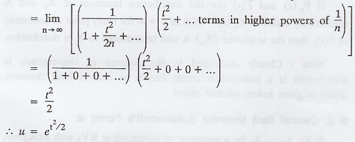
.'. By using uniqueness property of m.g.f, the variate. Z must be a standard normal variate as n → ∞

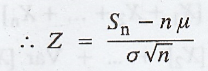
.'. S_n must be a normal variate having (mean = nµ) and (s.d - σ √ n)

Thus, as n → ∞, S_n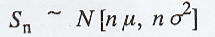 

Hence the proof.

Result 1:

Proof :

Result 2 :

ii. Convergence everywhere and almost everywhere

If {X_n} is a sequence of RVs and X is a RV such that it  = X, i.e., X_n → X as n → ∞, then the sequence {X_n} is said to converge to X everywhere.

If P {X_n → X} = 1 as n → ∞, then the sequence {X_n} is said to converge to X almost everywhere.

iii. Convergence in probability or Stochastic convergence

If P {|X_n - X| > ε} → 0 as n → ∞, then the sequence {X_n} is said to converge to X in probability.

As a particular case of this kind of convergence, we have the following result, known as Bernoulli's law of large numbers.

If X represents the number of successes out of 'n' Bernoulli's trials with probability of success P (in each trial), then {X/n} converges in probability to P.

i.e., P{|X/n - P| > ε} →  0 as n → ∞

iv. Convergence in the mean square sense

If E{|X_n - X|²} → 0 as n → ∞ then the sequence {X_n} is said to converge to X in the mean square sense.

v. Convergence in distribution

If F_n(x) and F(x) are the distribution functions of X_n and X respectively such that F_n(x) → F(x) as n → ∞ for every point of continuity of F(x), then the sequence {X_n} is said to converge to X in distribution.

Note: Closely associated to the concept of convergence in distribution is a remarkable result known as central limit theorem, which is given below without proof.

vi. Central limit theorem (Liapounoff's Form)

If X₁, X₂, ... X_n be a sequence of independent RVs with E(X_i) =µ_¡ and Var(X_i) = , i = 1, 2, ... n and if S_n = X₁ + X₂ + ... + X_n then under certain general conditions, S_n follows a normal distribution with mean 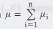 and Variance = 

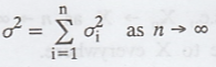
vii. Central limit theorem (Lindberg-Levy's form) [A.U A/M 2019 (R17) PQT]

If X₁, X₂, ... X_n be a sequence of independent identically distributed RV's with E (X_i) = µ and Var (X_i) = σ², i = 1, 2, ... n and if S_n = X₁ + X₂ + ... + X_n, then under certain general conditions, S_n follows a normal distribution with mean nµ  and variance nσ² as n → ∞

viii. Corollary

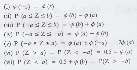
ix. Normal area property

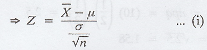
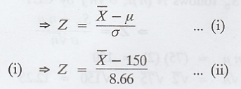
The normal variable 'Z' is defined as Z = X - µ / σ

Note that E(Z) = 0; V(Z) = 1. The std. normal distribution is 

P (0 < Z < 2) =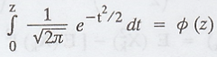 

x. Uses of Central Limit Theorem

(a) It is very useful in statistical surveys for a large sample size. It helps to provide fairly accurate results.

(b) It states that almost all theoretical distributions converge to normal distribution as n → ∞

(c) It helps to find out the distribution of the sum of a large number of independent random variables.

(d) It also helps explain the remarkable fact that the emprical blod frequencies of so many natural populations exhibit bell shaped (i.e. normal) curves.

Theorem :

Show that the central limit theorem holds good for a sequence {X_k}, if

Proof:

We have to verify that the condition given in the above note is satisfied by the given sequence {X_k}.

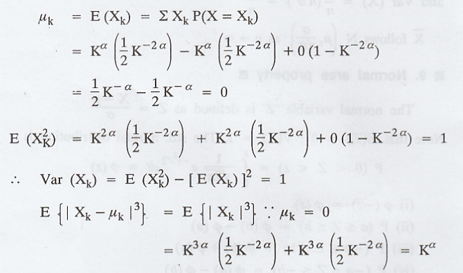
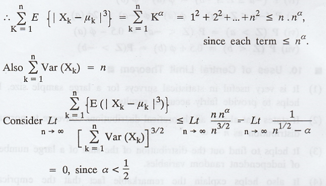
(i.e.,) the necessary condition is satisfied. Therefore CLT holds good for the sequence {X_k}.

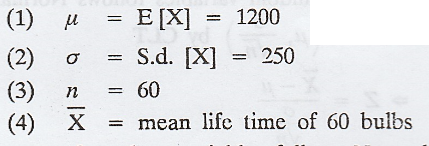
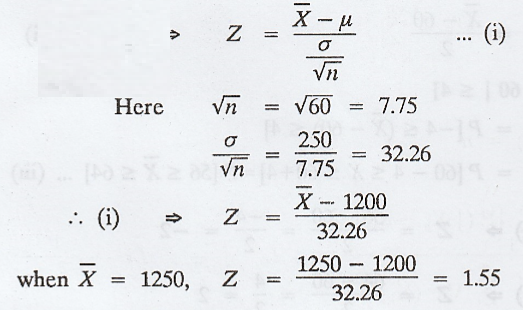
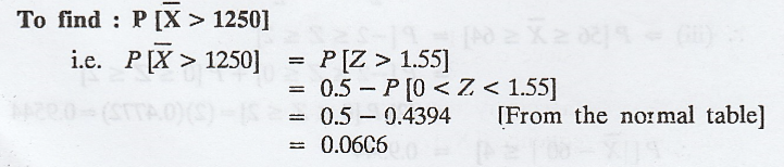
Example 2.5.a(1)

The lifetime of a certain brand of an electric bulb may be considered as a RV with mean 1200 h and standard deviation 250 h. Find the probability, using central limit theorem, that the average lifetime of 60 bulbs exceeds 1250 h. [AU N/D 2008] [AU N/D 2006] [A.U Trichy M/J 2011] [A.U N/D 2013] [A.U N/D 2018 R-17 PS]

Solution:

Given:

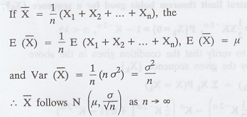
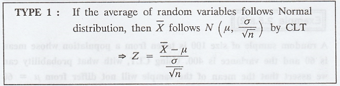
If the average of random variables follows Normal distribution, then X follows N (µ, σ/√n) by CLT

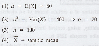
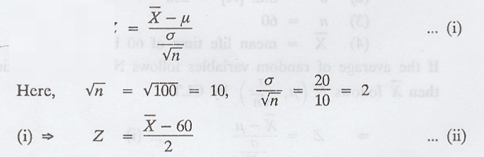
Example 2.5.a(2)

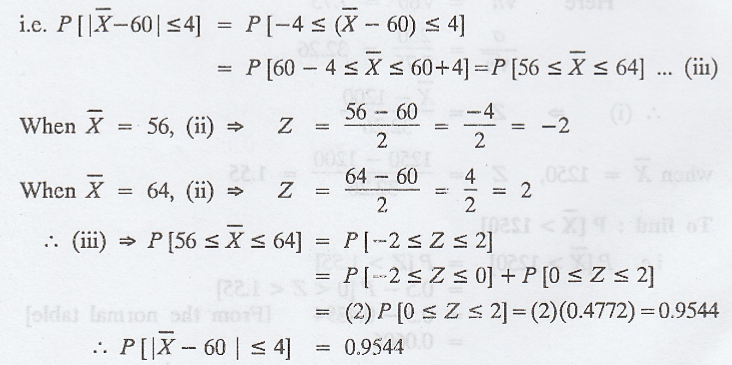
A random sample of size 100 is taken from a population whose mean is 60 and the variance is 400. Using CLT, with what probability can we assert that the mean of the sample will not differ from µ = 60 by more than 4? [AU A/M 2003, Trichy A/M 2010] [A.U A/M 2010] A.UA/M 2010

Solution:

Given: 

If the average of random variables follows Normal distribution, then X follows N (µ, σ/√n) by CLT

(ii) To find P [|X - 60 | = 4]

Example 2.5.a (3)

A distribution with unknown mean u has variance equal to 1.5. Use central limit theorem to find how large a sample should be taken from the distribution in order that the probability will be atleast 0.95 that the sample mean will be within 0.5 of the population mean. [A.U N/D 2013] [A.U. N/D 2004] [A.U A/M 2003]

Solution:

Given (1) Mean = µ

(2) σ² = 1.5 => σ = √1.5

(3) n

(4)  → Sample mean

If the average of random variables follows Normal distribution, then X follows N (µ, σ / √n) by CLT

To find 'n' such that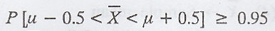 

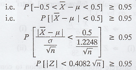
Where Z is the standard normal variate.

The least value of n is obtained from

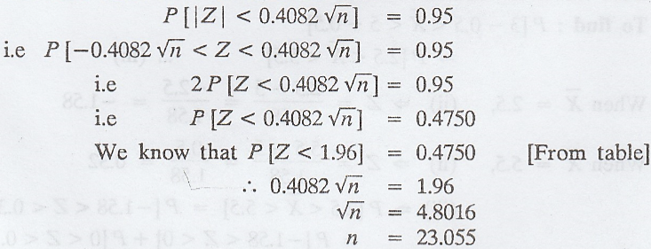
Therefore, the size of the sample must be atleast 24.

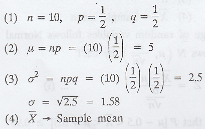
Example 2.5.b(1)

A coin is tossed 10 times. What is the probability of getting 3 or 4 or 5 heads. Use central limit theorem. [AU N/D 2009] [A.U CBT M/J 2010] [A.U N/D 2003]

Solution:

Given:

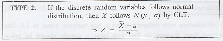
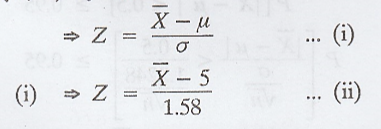
If the discrete random variables follows normal distribution, then eeeee follows N (µ, σ) by CLT.

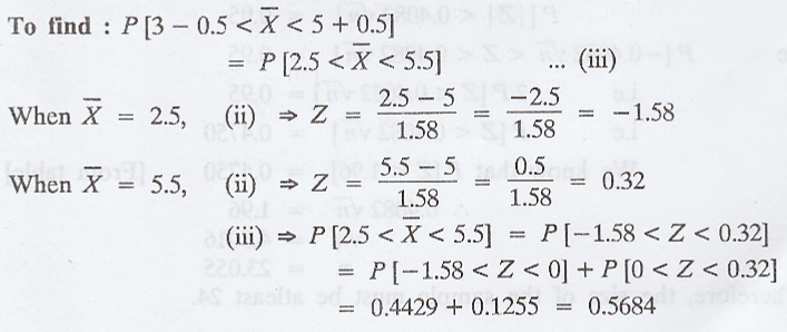
To approximate the discrete probability distribution to continuous probability distribution add 0.5 to the upper bound and subtract 0.5 from the lower bound.

Example 2.5.b(2)

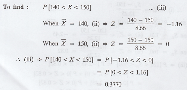
A coin is tossed 300 times found the probability that heads will appear more than 140 times and less than 150 times. [A.U Tvli M/J 2010]

Solution:

Given:

If the discrete random variables follows normal distribution, then  follows N (µ, σ) by CLT.

Example 2.5.c(1)

If X₁, X₂ ... X_n are Poisson variates with parameter λ = 2, use the central limit theorem to estimate P (120 ≤ Sn ≤ 160), where S_n = X₁ + X₂ + ... + X_n and n = 75. [AU N/D 2009, N/D 2010] [A.U M/J 2012]

Solution:

Given:

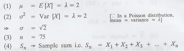
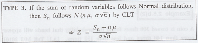
If the sum of random variables follows Normal distribution, then S follows N (nµ, σ√n) by CLT

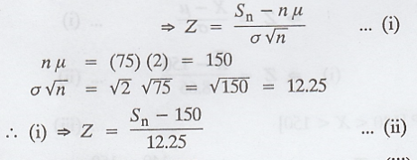
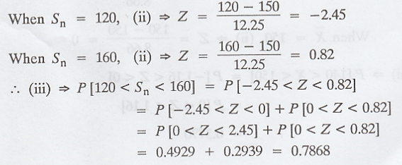
To find P[120 < S_n < 160]

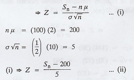
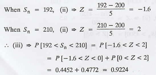
Example 2.5.c(2)

Let X₁, X₂ ..., X₁₀₀ be independent and identically distributed RVS with mean µ = 2 and σ² = 1. Find P(192 < X₁ + X₂+ ... + X₁₀₀ < 210) [A.U N/D 2012]

Solution:

Given:

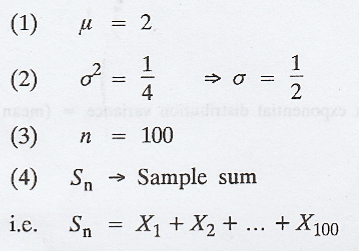
If the sum of random variables follows Normal distribution, then Sn follows N (nµ, σ√n) by CLT

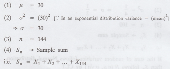
Example 2.5.c(3)

The burning time of a certain type of lamp is an exponential random variable with mean 30 hrs. What is the probability that 144 of these lamps will provide a total of more than 4500 hrs of burning time? [SIOS GM U.A] [A.U Trichy M/J 2011]

Solution:

Given:

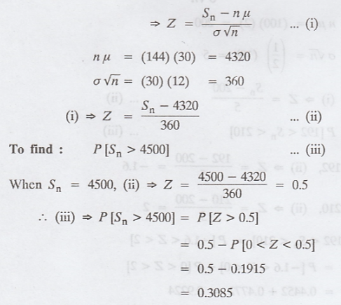
If the sum of random variables follows Normal distribution, then Sn follows N (nµ, σ√n) by CLT

Example 2.5.c(4)

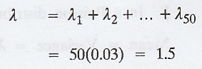
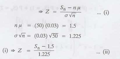
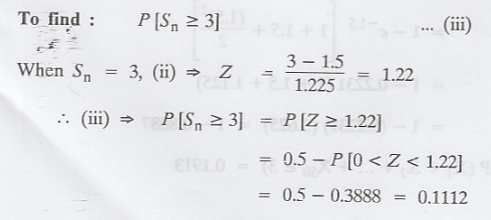
If X_i, i = 1, 2, ..., 50 are independent random variables each having a poisson distribution with parameter λ = 0.03 and S_n = X₁ + X₂ + ... + X_n, evaluate P (S_n ≥ 3) using CLT. Compare your answer with the exact value of the probability.

Solution:

Given:

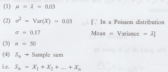
If the sum of random variables follows Normal distribution, then S follows N (nµ, σ√n) by CLT

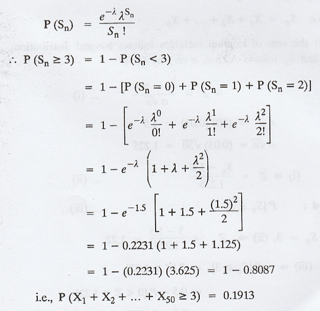
To find the exact value of P [X₁ + X₂ + ... + X₅₀ ≥ 3]

Here, X₁, X₂,..., X₅₀ are all independent Poisson variates with parameters,

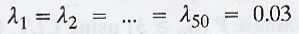
Hence, by the additive property of Poisson distribution,

.. The p.m.f of S_n is given by

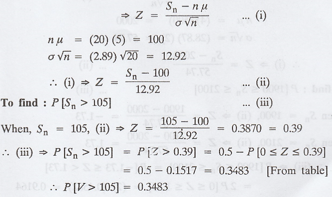
Example 2.5.c(5)

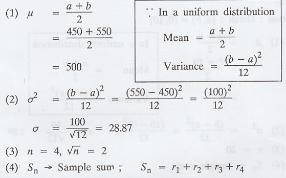
The resistors r₁, r₂, r₃ and r₄ are independent random variables and is uniform in the interval (450, 550). Using the central limit theorem find P (1900 = r₁ + r₂ + r₃ + r₄ ≤ 2100)

Solution:

Given: (a, b) = (450, 550)

If the sum of random variables follows Normal distribution, then Sn follows N (nµ, σ√n) by CLT

Example 2.5.c(6)

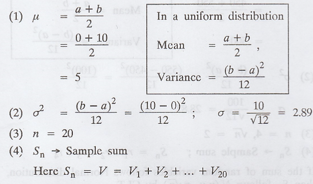
If V_i, i = 1, 2, 3, ... 20 are independent noise voltages received from 'adder' and V is the sum of the voltages received, find the probability that the total incoming voltage V exceeds 105, using CLT. Assume that each of the random variables V_i is uniformly distributed over (0, 10)

Solution:

Given: (a, b) = (0, 10)

If the sum of random variables follows Normal distribution, then S follows N (nµ, σ√n) by CLT

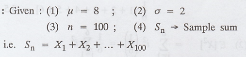
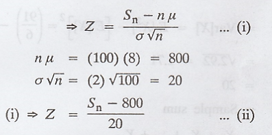
Example 2.5.c(7)

Suppose that orders at a restaurent are identically independent randem variables with mean µ = 8 and standard deviation σ = 2.

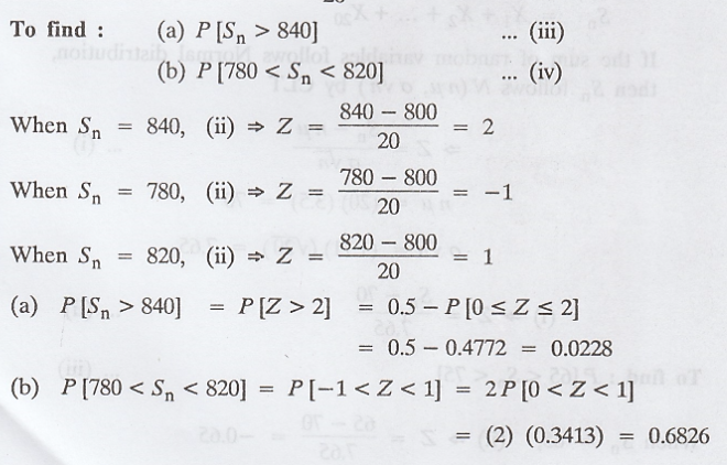
Estimate

(a) The probability that first 100 customers spend a total of more than 840

(b) P [780 < X₁ + X₂ + ... + X₁₀₀ < 820] [A.U. A/M 2008]

Solution:

If the sum of random variables follows Normal distribution, then S, follows N (nµ, σ√n) by CLT

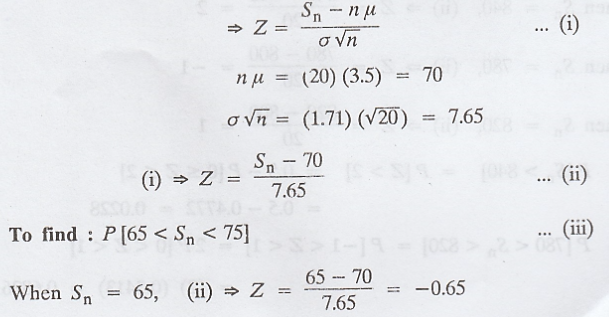
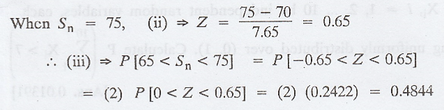
Example 2.5.c(8)

Twenty dice are thrown. Find approximately the probability that the sum obtained is between 65 and 75 using CLT.

Solution:

Given:

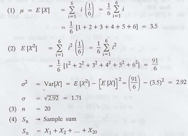
If the sum of random variables follows Normal distribution, then S_n follows N (nµ, σ√n) by CLT

EXERCISE 2.5

1. The guaranteed average life of a certain type of electric light bulb is 1000 h with a S.D. of 125 h. It is decided to sample the output so as to ensure that 90% of the bulbs do not fall short of the guarnteed average by more that 2.5%. Use CLT to find the Jon minimum sample size?

2. If X_i, i 1, 2... 50 are independent RVs, each having a poisson distribution with parameter λ = 0.03 and S_n = X₁ + X₂ + X_n find P (S_n ≥ 3) using CLT. Compare your answer with the exact value of the probability.

3. A random sample of size 100 is taken from a population whose mean is 60 and variance is 400. Using CLT with what probability can we assert that the mean of the sample will not differ from µ = 60 by more than 4 ?

4. Test whether the CLT holds good for the sequence {X_k} if P {X_k = ± 2^k} = 2^{-(2k + 1)}, P(X_k = 0) = 1 - 2^-2k

5. The lifetime of a special type of battery is a random variable with mean 40 hours and standard deviation 20 hours. A battery is used until it fails, at which point it is replaced by a new one. Assuming a stockpile of 25 such batteries the lifetimes of which are independent, approximate the probability that over 1000 hours of use can be obtained. [Ans. 0.1587]

6. Let X₁, X₂, ... X₁₀ be independent Poisson random variable with Mean 1. Use the Central limit theorem to approximate P {X₁ + X₂ + ... + X₁₀ ≥ 15}.

7. Let X_i, i = 1, 2, ... 10 be independent random variables, each being uniformly distributed over (0, 1). Calculate 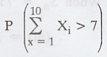 [Ans. 0.01391]

8. Let X be the number of times that a fair coin flipped 40 times, lands heads. Find the probability that X = 20. [Ans. 0.1272]

9. The guaranteed average life of a certain type of electric light bulb is 1000 h with a standard deviation of 125 h. It is decided to sample the output so as to ensure that 90% of the bulbs do not fall short of the guaranteed average by more than 2.5%. Use Central limit theorem to find the minimum sample size. [Ans. 41]