Block Diagram Representation

BLOCK DIAGRAM REPRESENTATION

The LTI system can also be represented with the help of block diagrams. Which indicates how individual calculations are performed.

Realization of Continuous-time Systems-(Direct Form I Realization)

There are four different types of system realization of continuous-time linear time invariant systems.

They are:

1. Direct form-I realization

2. Direct form-II realization

3. Cascade form realization

4. Parallel form realization

Integrator

An integrator is an element used to integrate the input signal. The transfer function of an ideal integrator is given by

Adder

The adder is an element used to perform the addition and subtraction of signals. Pictorially it is represented by a small circle that has at least two input terminals and one output terminal. The output variable is the algebraic sum of all the input variables.

Multiplier

The multiplier is an element used to multiply the signal by a constant. The gain can be positive or negative.

The transfer function of the system is

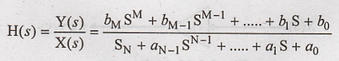
H(S) = Y(S)/X(S)

System Realization

There are different types of system realizations. They are 1. Direct form -I realization 2. Direct form-II realization 3. Cascade form realization 4. Parallel form realization. A transfer function can be realized using integrators and differentiators. However, differentiators are not used in realizing practical systems. The reason is that differentiators amplifies high frequency noise. The integrator suppress high frequency noise, hence only integrators are used for realization of systems.

The transfer function of ideal integrator is given by,

H(s) = 1/s

Below figure represents the transfer function of an ideal integrator

Consider a system defined by differential equation

The transfer function of above system is,

If M > N, the system is not causal, and the system is not physically realizable.

Therefore the value of M must be less than or equal to N of physical realizability.

Realization of Direct form I-Structure

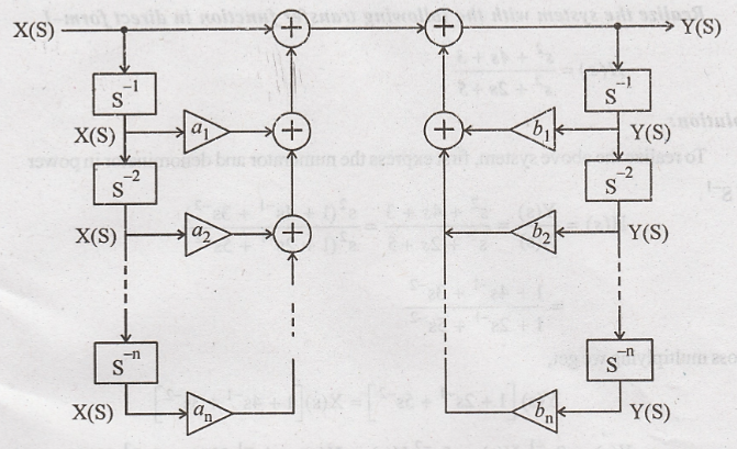
Realization of Direct form - II

Problem 1:

Realize the system with the following transfer function in direct form-I

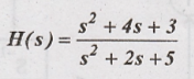
Solution:

To realize the above system, first express the numerator and denominator in power of S^-1.

Cross multiplying we get,

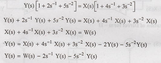
For this first we realized W(S) as shown in figure 3.4(a) then we realized Y(S) in terms of W(S) as shown in figure 3.4(b) combining figures 3.4(a) and 3.4(b) we get the realization as shown in figure 3.5.

Problem 2:

Realize the system with the following transfer function in direct form -I:

Solution:

Cross multiplying we get,

The direct form -I realization of Y(s) is shown in figure 3.6

Problem 3:

Realize the system described by the following differential equation in direct form-1. 

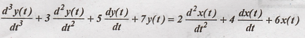
Solution:

Given:

Taking Laplace transform on both sides and neglecting initial conditions, we have 

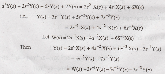
The realization of the given transfer function in direct form -I is shown in fig. 3.7.